Mechanical Engineering Portfolio

Precision engineering
from theory to reality.

Six projects spanning manufacturing, controls, sensing, structural analysis, and reverse engineering — combining first-principles calculations, physical builds, computational analysis, and documented testing where appropriate.

0
Projects
±0″
Tightest Tolerance
$0K+
Projected Savings
0
Prototypes Machined
0
Documented Inspection Characteristics

Engineering Projects

Five additional projects spanning control systems, biomedical sensing, structural analysis, precision manufacturing, and mechanical reverse engineering.

Project 02

PPG Heart Rate Monitor

MAX30102 + Arduino Uno — Optical Biosensing & Signal Processing

Built an Arduino-based optical sensing system around the MAX30102 to acquire Red/IR reflectance signals and explore heart-rate extraction, filtering, numerical differentiation, and comparison with reference readings.

MAX30102
Optical Biosensor
Red + IR
Dual Channels
~25 Hz
Logged Cadence
2
Reference Comparisons
Hardware & Assembly
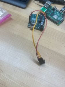
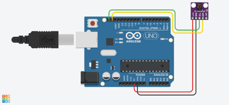
Arduino Uno with MAX30102 breakout
Arduino Uno with MAX30102 breakout used for optical acquisition.

Embedded Sensor Integration

The MAX30102 is an integrated heart-rate / pulse-oximetry biosensor with red and IR emitters. It was interfaced to an Arduino Uno over I2C, acquiring Red/IR reflectance channels for signal-processing experiments.

  • Dual-channel Red + IR acquisition over I2C
  • Moving-average filtering of the raw optical signal
  • Derivative-based peak-detection concept for heartbeat identification
  • MAX30102 configured for 100-Hz acquisition; the saved/displayed analysis data show approximately 25-Hz effective sample cadence
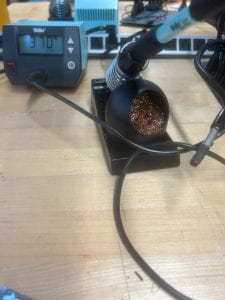
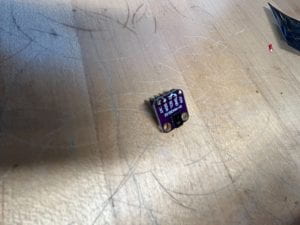
Soldering setup during sensor prototype assembly
Soldering setup used during sensor-prototype assembly.

Prototype Assembly

Header connections were soldered and continuity checked before powering. The breadboard platform allowed rapid iteration on sensor positioning and finger placement during testing.

Raw Signal Acquisition
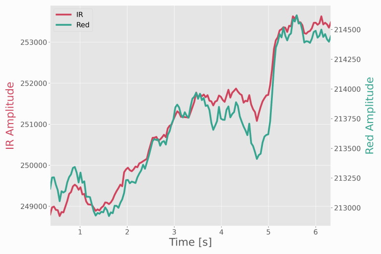
Raw Red/IR optical signal during resting acquisition
Raw Red/IR optical signal during the resting acquisition. Large DC baseline and drift are visible; this is not presented as a detrended pulse morphology plot.

Resting Acquisition

The resting trace shows the raw Red/IR reflectance with a large DC baseline and visible drift. Heart-rate estimates were extracted from the moving-average-filtered signal using the derivative-based peak detector.

Project-recorded estimate: 72.4 BPM at rest.

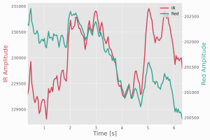
Raw Red/IR optical signal after exercise
Raw Red/IR optical signal after exercise; displayed as raw optical sensor data rather than a clinical PPG morphology trace.

Post-Exercise Acquisition

After exercise the oscillation visibly speeds up while the raw trace retains the same DC-baseline and drift characteristics. Project-recorded estimate: 124.6 BPM post-exercise.

Formal HRV/PRV analysis was outside the scope of this short acquisition; robust HRV typically requires beat-to-beat interval analysis over a substantially longer record.

Reference Comparison

Single-Session Reference Comparison

ConditionSensor EstimateReferenceAbs. Difference
Resting72.4 BPM74 BPM1.6 BPM
Post-exercise124.6 BPM126 BPM1.4 BPM

Single-session comparison; not a population-level accuracy validation.

Numerical Signal Processing

The processing chain — acquire → filter → differentiate → threshold → count peaks — was implemented as a numerical exercise on the logged data.

Trapezoidal integration was applied as a numerical signal-area exercise. Because raw PPG amplitude depends strongly on sensor contact, optical geometry and tissue, the integral is not interpreted as cardiac work or cardiac output.

Circuit Diagram & Data

The project demonstrated embedded optical sensing, I2C acquisition, basic digital filtering, numerical signal processing, and the importance of validating analysis against the actual recorded dataset.

Signal Processing PPG / Biosensing I2C / Embedded Data Analysis Filtering / Peak Detection Biomedical
Project 03

Stress Concentration Around a Circular Hole

Kirsch Analytical Solution + Python Numerical Visualization + Arduino Sensor Experiment

Analyzed the classical stress-concentration problem — a circular hole in a tensile plate — using the Kirsch analytical solution, a Python numerical evaluation of that solution over a computational grid, and a separate Arduino strain-sensor acquisition experiment.

Kt = 3
Kirsch SCF (Infinite Plate)
500×500
Python Numerical Grid
d/W = 0.25
Finite-Width Specimen
Arduino
Sensor Acquisition
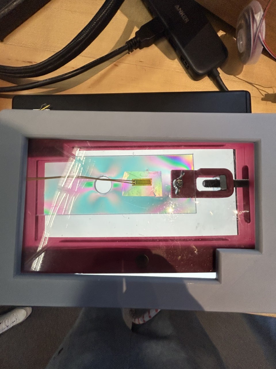
Actual stress opticon — physical experimental setup
The actual stress opticon — physical experimental setup for the stress concentration project.

Project Overview

Analyzed the classical stress-concentration problem — a circular hole in a tensile plate — using the Kirsch analytical solution, a Python numerical evaluation of that solution over a computational grid, and a separate Arduino strain-sensor acquisition experiment.

1. Analytical Kirsch Solution
Kirsch stress distribution around a circular hole
Kirsch analytical stress distribution around a circular hole under uniaxial tension.

Kirsch Analytical Solution

For an infinite plate with a circular hole under uniaxial remote tension, the Kirsch solution predicts a maximum hoop stress of 3σ∞ at the hole boundary at θ = ±90°:

Kt = σmax / σ∞ = 3 ANALYTICAL

Important limitation: the physical specimen had d/W = 12.5/50 = 0.25, so finite-width effects are not negligible. Kt = 3 is used as the classical infinite-plate reference, not asserted as the exact finite-specimen factor.

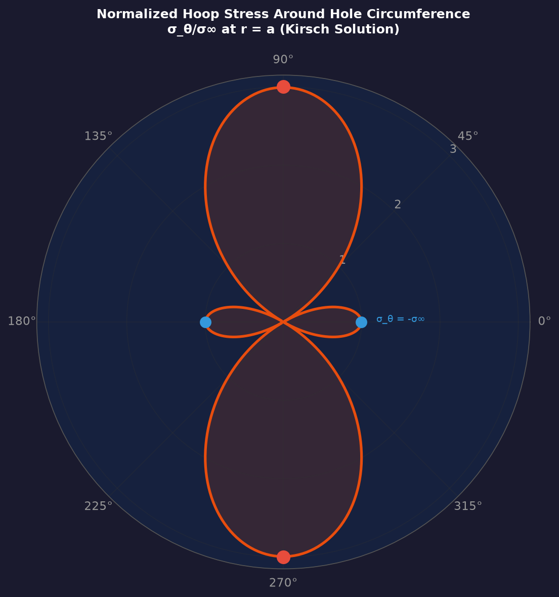
Polar representation of the Kirsch stress field
Polar representation of the Kirsch stress field — angular dependence of hoop stress at the hole boundary.

Stress Orientation

The maximum tensile hoop stress occurs at the hole boundary at points perpendicular to the applied loading axis (θ = ±90°) — the hole interrupts the load path and the material around it must redistribute that stress.

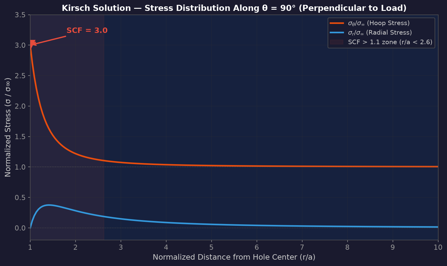
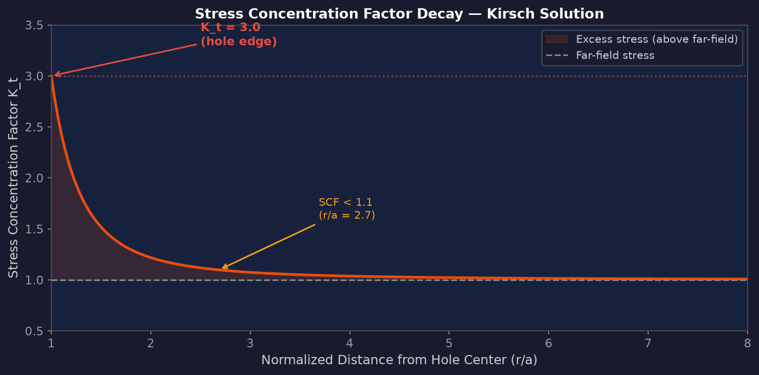
Stress concentration factor decay from hole edge
Normalized hoop stress decay in the infinite-plate Kirsch field as a function of r/a.

Decay with Distance

In the infinite-plate Kirsch field, the normalized stress falls below approximately 1.1 by r/a ≈ 2.7 — the concentration decays quickly away from the hole edge, though the exact decay on the finite specimen differs from the infinite-plate curve.

2. Python Numerical Visualization
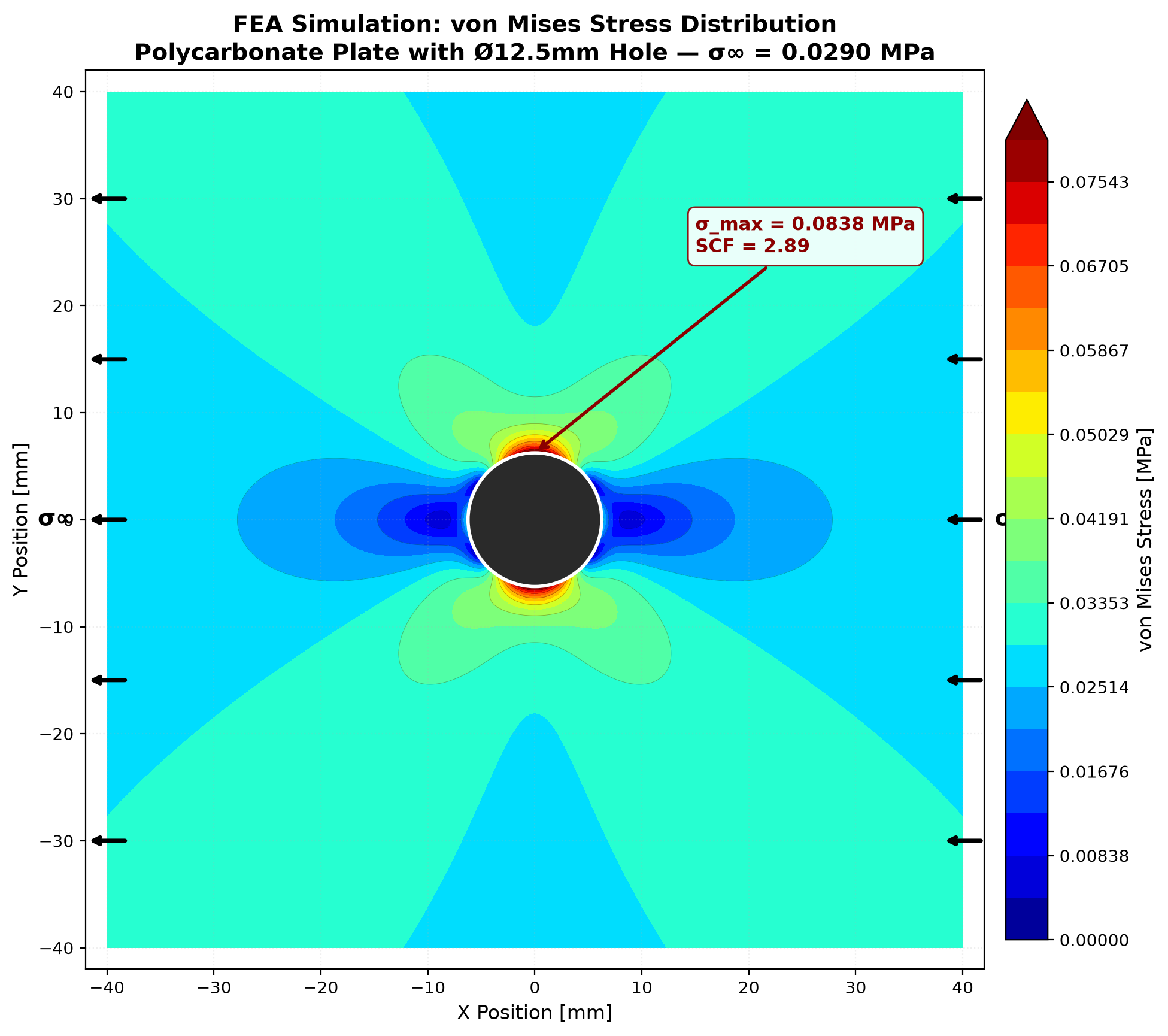
Python numerical evaluation — Kirsch-derived von Mises stress field
Python Numerical Evaluation — Kirsch-derived von Mises stress field over the 500×500 computational grid.

Numerical Evaluation of the Kirsch Field

The analytical Kirsch equations were evaluated directly in Python (NumPy) over a 500×500 computational grid to visualize the full stress field — σr, σθ, τrθ — and derived quantities such as von Mises and principal stresses, all transformed from the same analytical solution.

This is a numerical evaluation of a closed-form solution, not a finite-element analysis. No mesh, no solver, no discretization error study — the grid simply samples the exact equations for plotting.

Output from the Python code — numerical evaluation of Kirsch stress field
Output from the Python code — numerical evaluation showing computed stress values across the grid.

Code Output

The Python script evaluates the Kirsch equations across the grid and outputs the computed stress field values. The von Mises stress is derived from the analytical stress components using the standard transformation:

σvm = √[ ½((σr − σθ)² + σr² + σθ² + 6τrθ²) ]

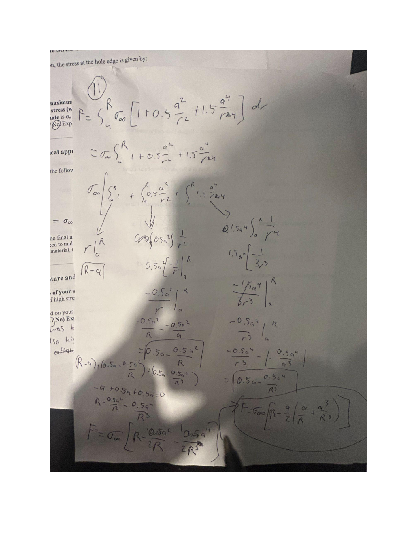
Derived formula for force integration across the net section
Derived formula — integrating the Kirsch hoop stress over the finite-width ligament to check force equilibrium.

Derived Formula & Force Check

As a consistency check, the truncated Kirsch hoop stress at θ = 90° was integrated over the two ligaments of the finite-width section CALCULATED:

σθ(r) = σ∞ [ 1 + a²/(2r²) + 3a⁴/(2r⁴) ]
FK = 2 t σ∞ [ R − a²/(2R) − a⁴/(2R³) ]

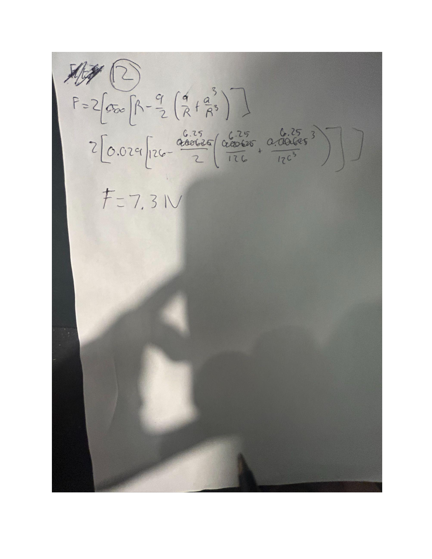
Values plugged into the derived force equation
Values plugged into the derived equation — with W=50 mm, t=3 mm, a=6.25 mm, R=25 mm, and σ∞=0.029 N/mm².

Notes on the Force Calculation

With W = 50 mm, t = 3 mm, a = 6.25 mm, R = W/2 = 25 mm, and σ∞ = 0.029 N/mm²:

FK ≈ 4.21 N versus the gross far-field resultant F∞ = σ∞ W t = 4.35 N — about a 3.3% difference, illustrating the limitation of applying the infinite-plate solution at a nearby finite boundary. This is an analytical consistency check, not experimental validation.

3. Arduino Strain-Sensor Experiment

Sensor Acquisition & Strain Gauge Data

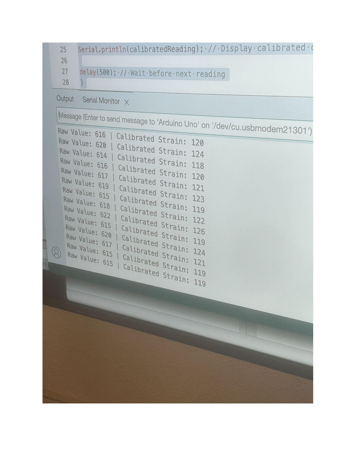
An Arduino / Wheatstone-bridge experiment was built to acquire strain-sensor output near the hole. The strain gauge was bonded near the hole boundary at θ = ±90° where the Kirsch solution predicts maximum hoop stress.

The archived calibration implementation was not sufficient for a defensible absolute microstrain measurement, so the experiment is presented as a sensor-acquisition exercise rather than quantitative validation of the Kirsch SCF.

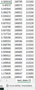
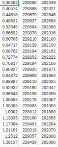
Raw ADC readings were logged during load application and compared against the expected strain signal direction. The gauge responded in the correct direction (tension at the predicted location), confirming sensor functionality and signal chain integrity PROJECT RECORD.

The lesson: instrumentation results must be verified against a sound calibration chain before they can be treated as measurement evidence.

The project demonstrates elasticity theory, coordinate stress transformation, numerical visualization, and experimental instrumentation — while also showing why computational and sensor methods must be independently validated before being treated as quantitative evidence.

Elasticity Kirsch Solution Python / NumPy Stress Analysis Arduino Instrumentation
Project 04

PID Self-Balancing Robot

Inverted Pendulum — Arduino Uno + MPU-6050 + Dual NEMA 17 Steppers

Built and tuned a two-wheeled self-balancing robot using an Arduino Uno, MPU-6050 IMU, A4988 stepper drivers, and discrete PID control. The project focused on how proportional, integral, derivative, and sampling behavior affect stability in an inverted-pendulum system.

The system is conceptually related to other unstable attitude-control problems, although the actuator, dynamics, sensing, and control architecture are very different.

Arduino Uno
Controller
MPU-6050
6-DOF IMU
PID
Closed-Loop Control
Kp 4 / Ki .08 / Kd 3
Final Recorded Gains
Robot & Circuit Design
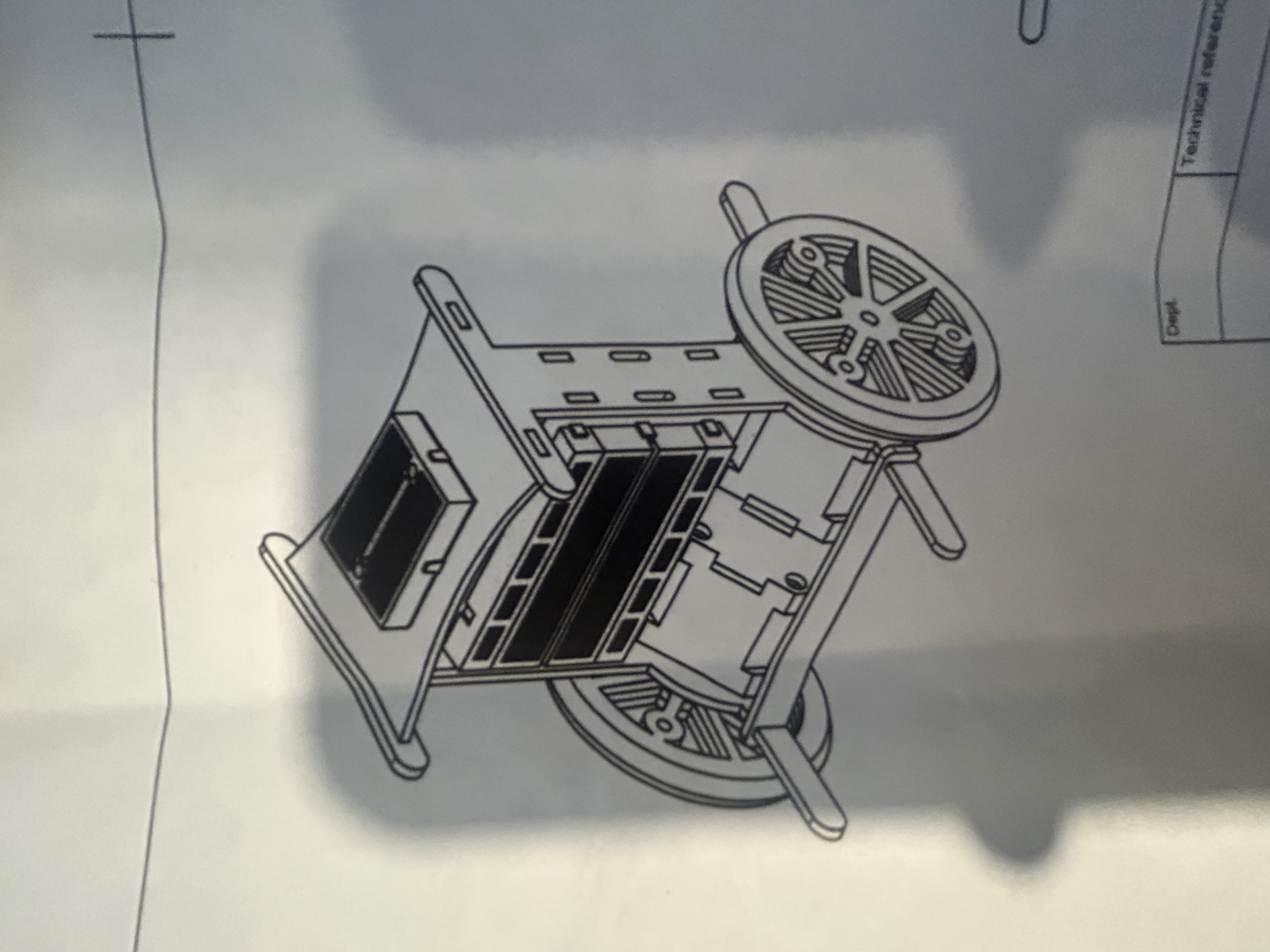
Mechanical design drawing of the self-balancing robot chassis
Mechanical design drawing for the self-balancing robot chassis.

System Architecture

The control challenge is the classical inverted pendulum: an inherently unstable system that tips over without continuous corrective actuation.

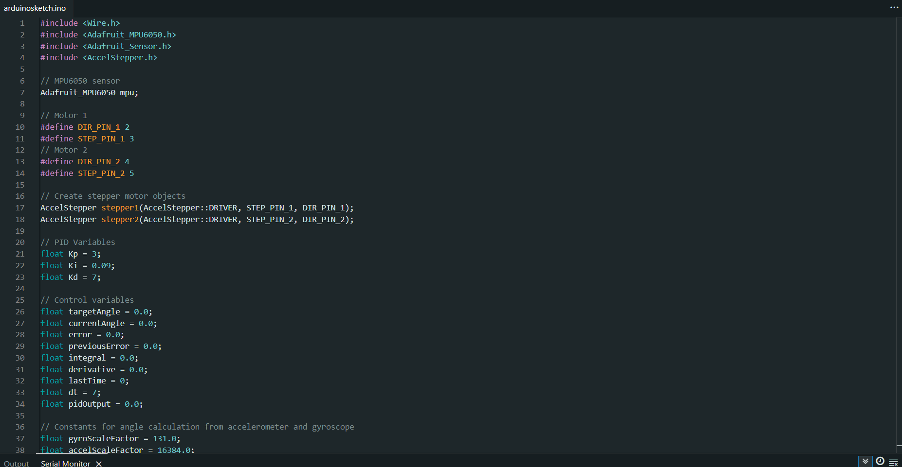
  • Controller: Arduino Uno running discrete PID with anti-windup / integral limiting
  • Sensing: MPU-6050 6-DOF IMU, gyro+accelerometer combined with a complementary-filter approach
  • Actuation: Two NEMA 17 stepper motors driven by A4988 drivers
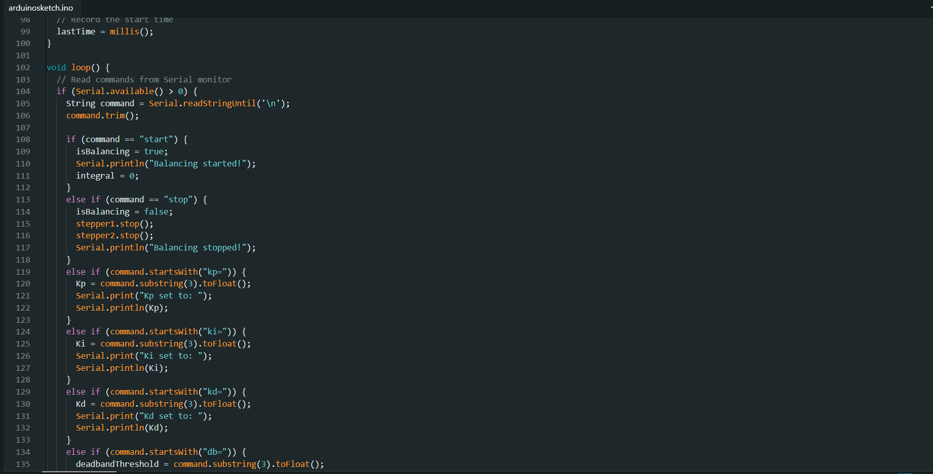
  • Tuning: Serial gain adjustment without reflashing firmware
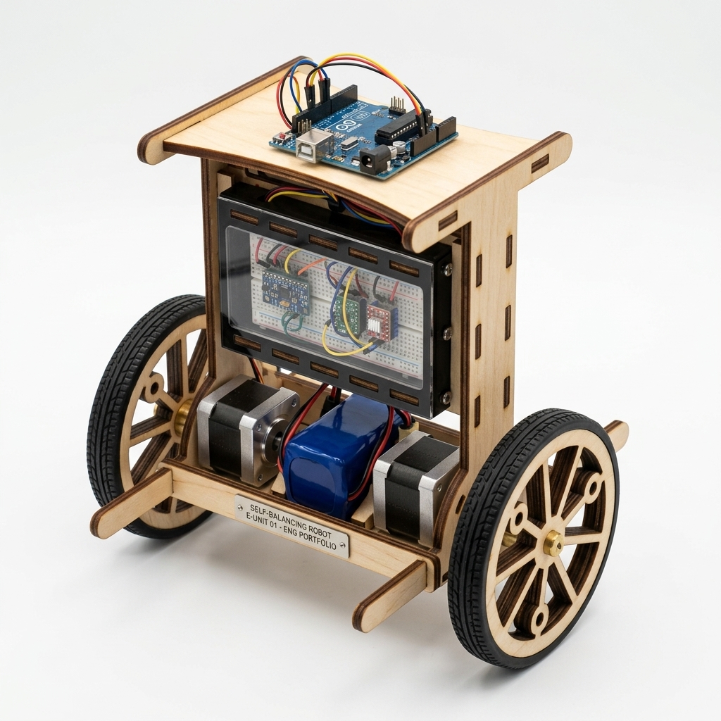
Concept design visualization of the two-wheeled balancing platform
CONCEPT / RENDER Design visualization of the two-wheeled balancing platform and component layout.

Mechanical Design

Laser-cut plywood chassis with the component layout organized around the axle line. A CAD-based mass-distribution calculation placed the center of mass approximately 29.7 mm above the axle CALCULATED.

Battery placement and component stacking were chosen to shape the pendulum's response — a higher center of mass gives the controller more time to react before the robot falls.

Control Law

Discrete PID Control

u[k] = Kp e[k] + Ki Σ( e Δt ) + Kd ( e[k] − e[k−1] ) / Δt

Complementary-filter attitude estimate:

θ = α ( θprev + ω Δt ) + (1 − α) θaccel

Final tuning settled near Kp = 4, Ki = 0.08, Kd = 3 after qualitative iterative testing PROJECT RECORD. These gains are specific to this build and are not universal tuning values.

Implementation Notes

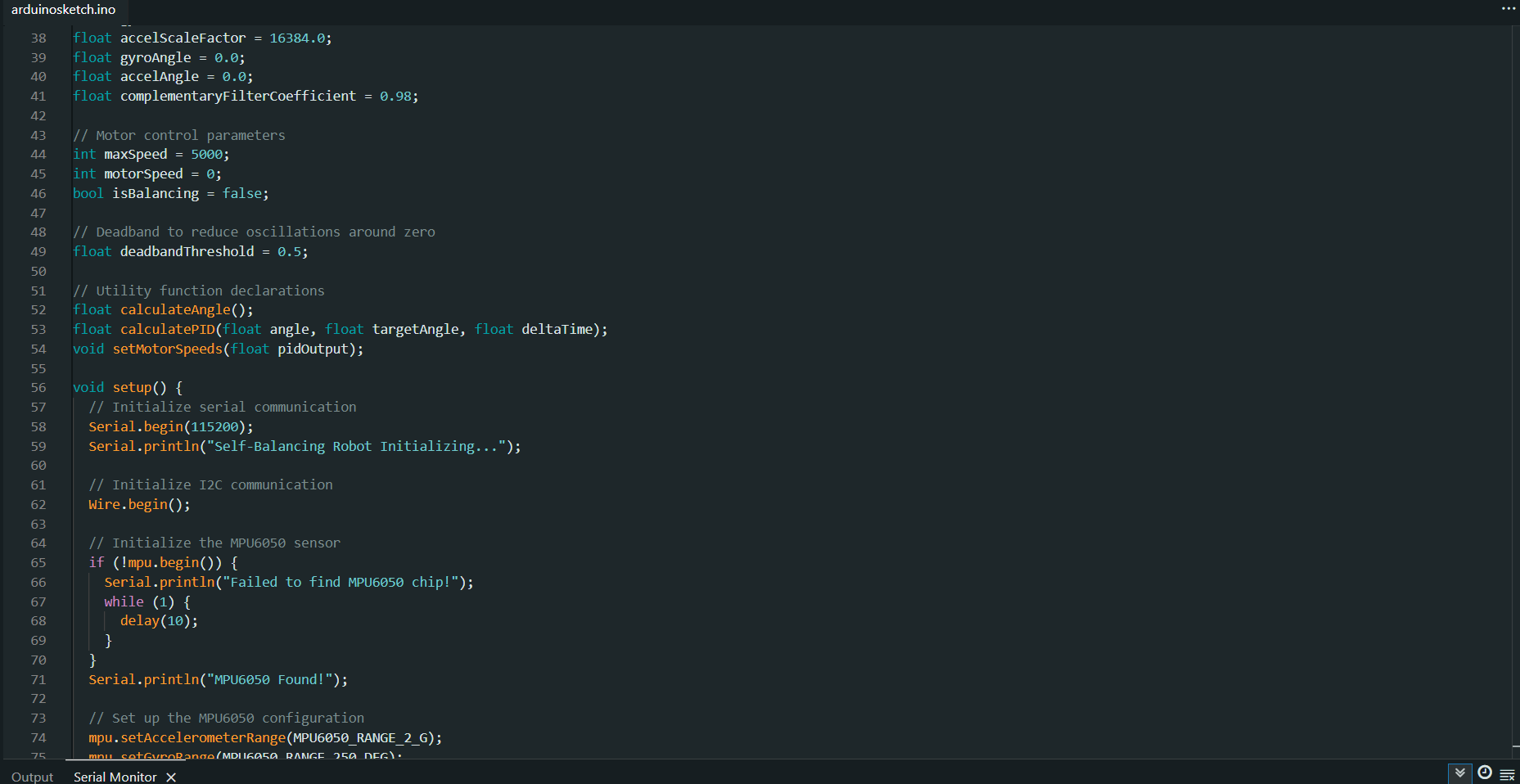
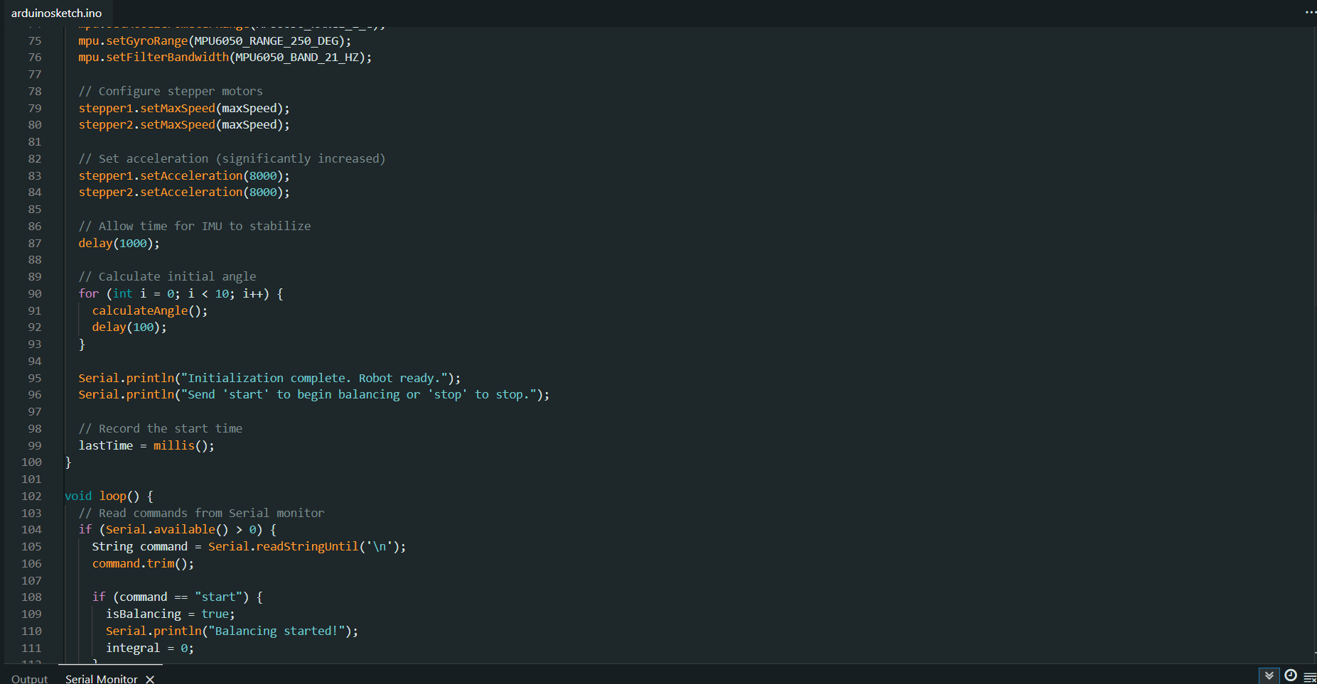
Archived firmware was used for iterative control testing; the portfolio focuses on the control architecture rather than claiming precise hard-real-time execution.

Tuning was performed through a serial command interface, allowing proportional, integral, and derivative gains to be adjusted during live balance testing without reflashing.

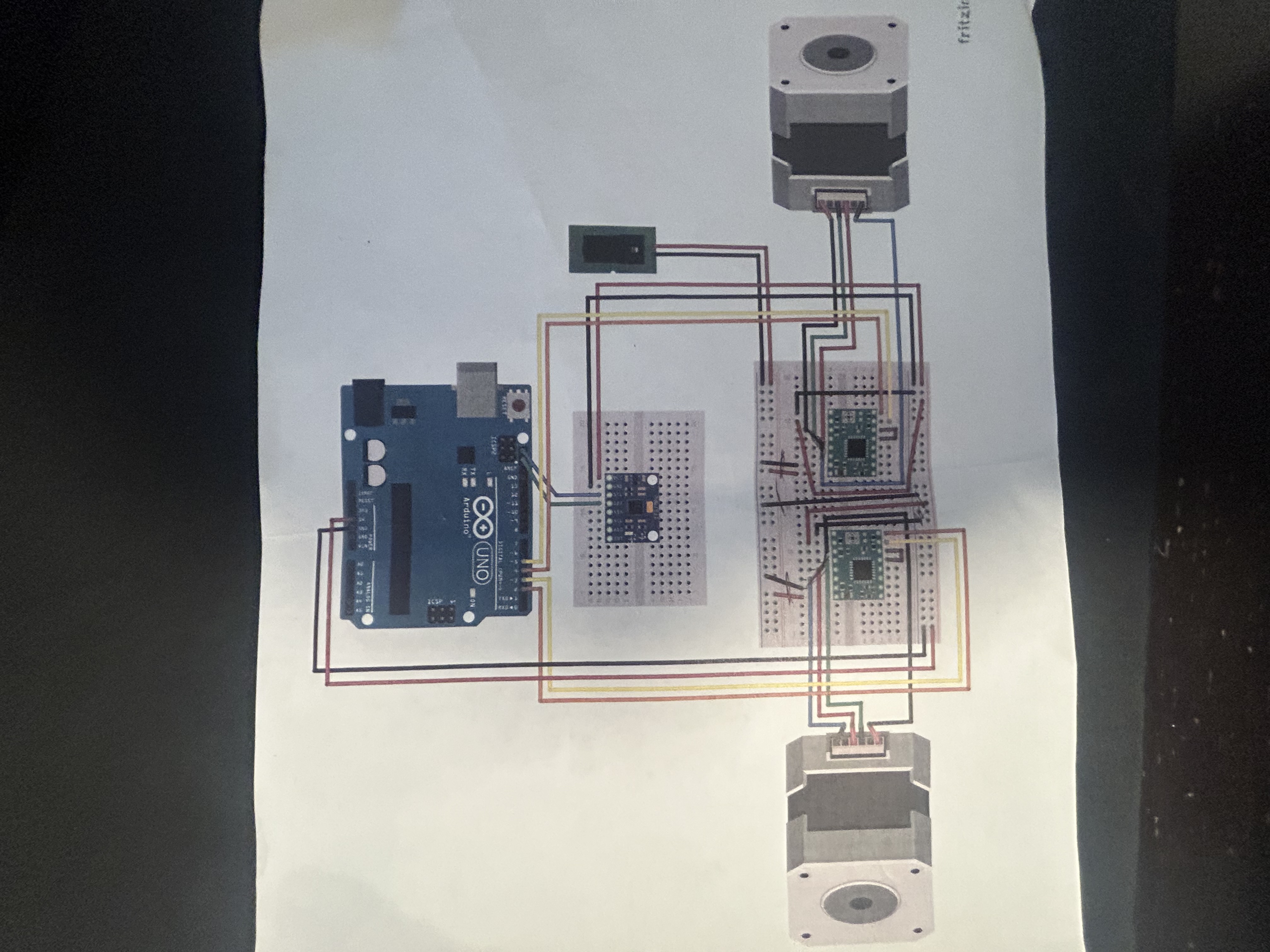
Wiring diagram for the balancing robot
Project wiring diagram showing Arduino, MPU-6050, A4988 drivers, and dual stepper motors.

Electrical Architecture

Arduino/logic power was separated from the higher-current stepper-motor power path to reduce coupling of motor noise into the sensor/control electronics.

Firmware
PID Tuning
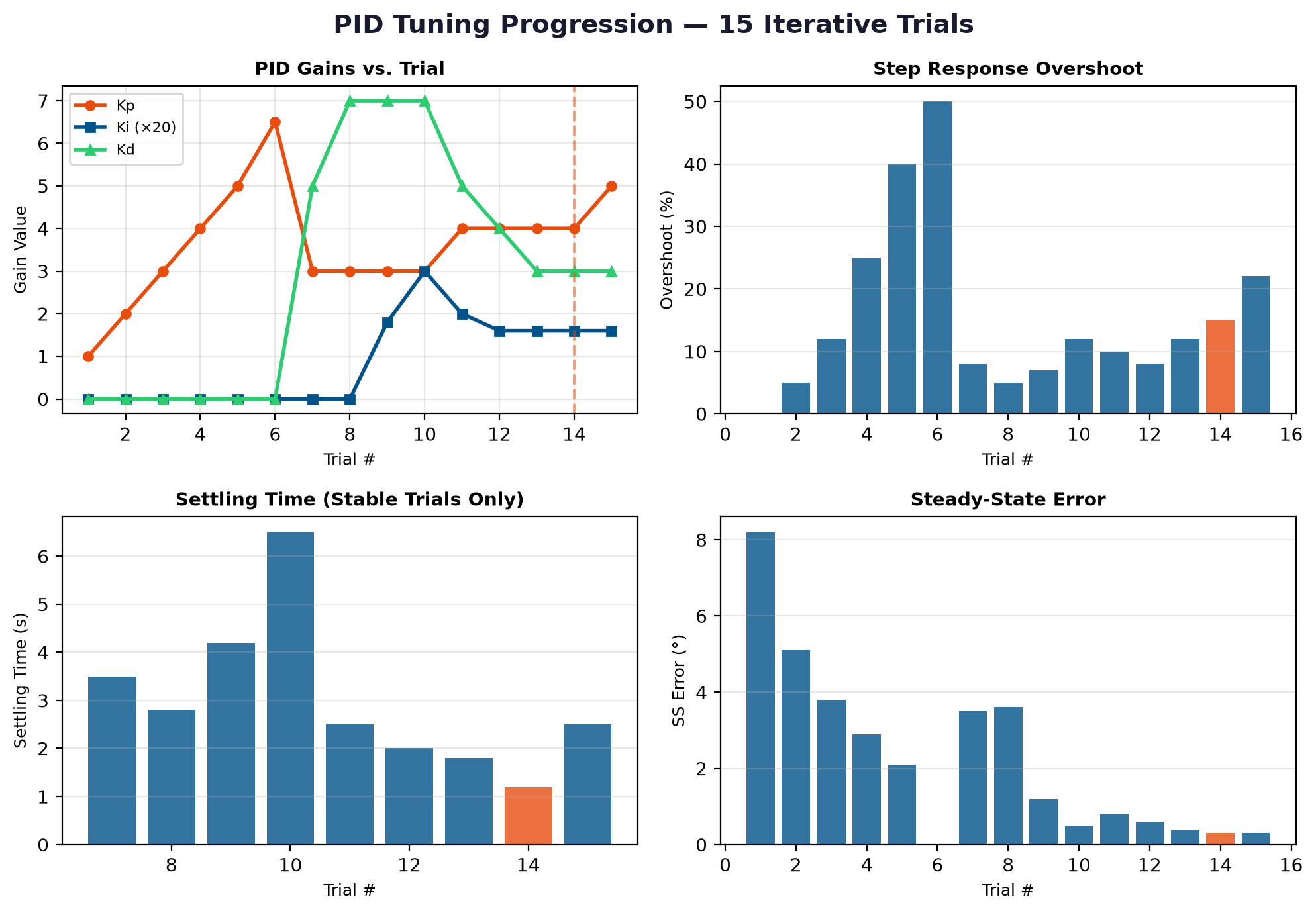
PID tuning chart — system response across different gain combinations
PID tuning chart — system response across different gain combinations during iterative testing.

Iterative Tuning Process

Tuning was performed through a serial command interface, allowing proportional, integral, and derivative gains to be adjusted during live balance testing without reflashing firmware.

The tuning process involved:

  • Starting with conservative gains and increasing Kp until the robot could maintain approximate balance
  • Adding Kd to damp oscillations and improve recovery from disturbances
  • Applying small Ki to correct steady-state lean from center-of-mass offset
  • Testing disturbance recovery by gently pushing the robot

Final tuning settled near Kp = 4, Ki = 0.08, Kd = 3 after qualitative iterative testing PROJECT RECORD. These gains are specific to this build and are not universal tuning values.

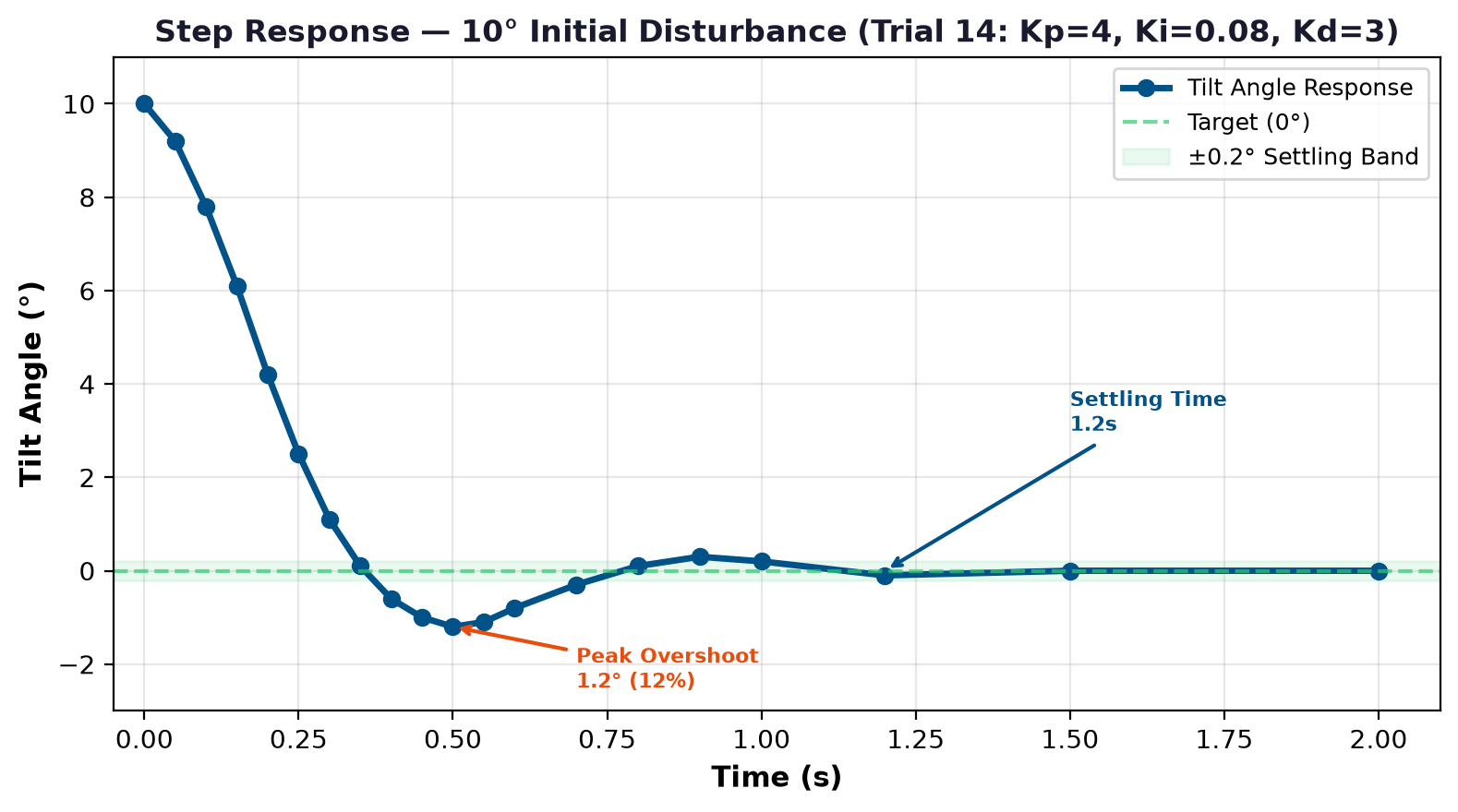
Step response — robot recovery from an applied disturbance
Step response — robot recovery from an applied disturbance during tuning.

Step Response & Stability

The step response shows how the robot recovers from an applied lateral disturbance. A well-tuned PID controller returns to equilibrium with minimal overshoot and no sustained oscillation.

Anti-windup / integral limiting was implemented to prevent integral accumulation from driving the steppers beyond their useful range during large tilt excursions.

PID Control Sensor Fusion Embedded C++ Arduino Control Theory Real-Time Systems
Project 05

CNC Precision Machining — Production Experience

American Precision Machining | Multi-Axis CNC | Metrology | Surface Finish

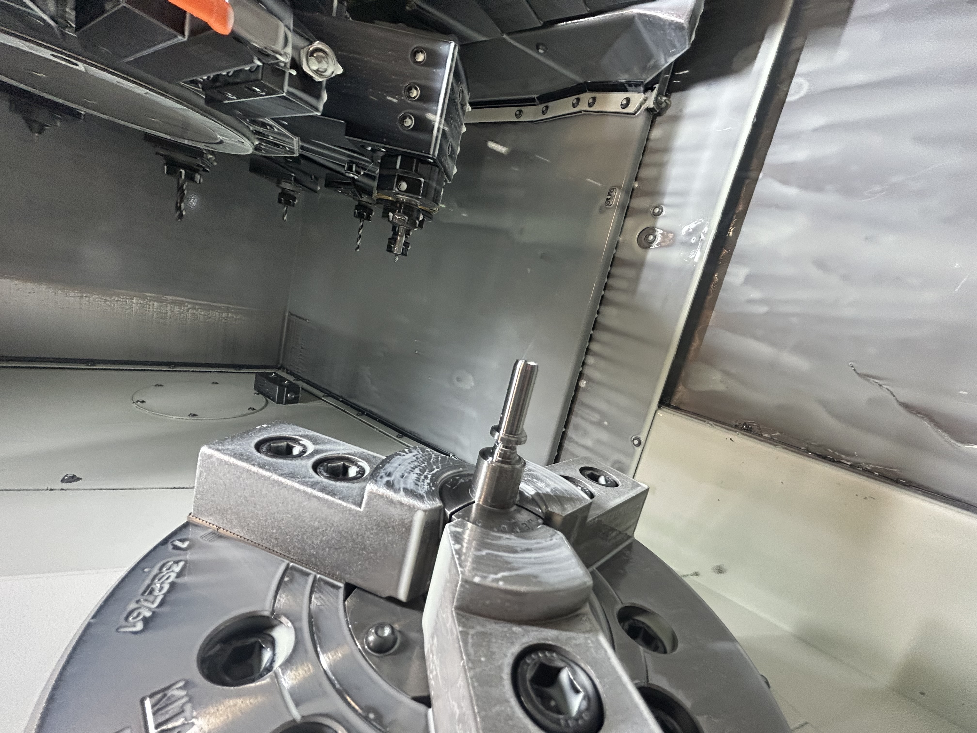
Production machining experience at American Precision Machining producing tight-tolerance components for industrial and instrumentation applications. Original customer drawings and programs are omitted for confidentiality; the project focuses on manufactured hardware, process knowledge, and documented inspection examples.

99%
QC Pass Rate
±0.0005"
Tightest Documented Tolerance
Ra 6.2
Best Documented Surface Finish (μin)
Multi-Axis
INTEGREX / CNC Experience
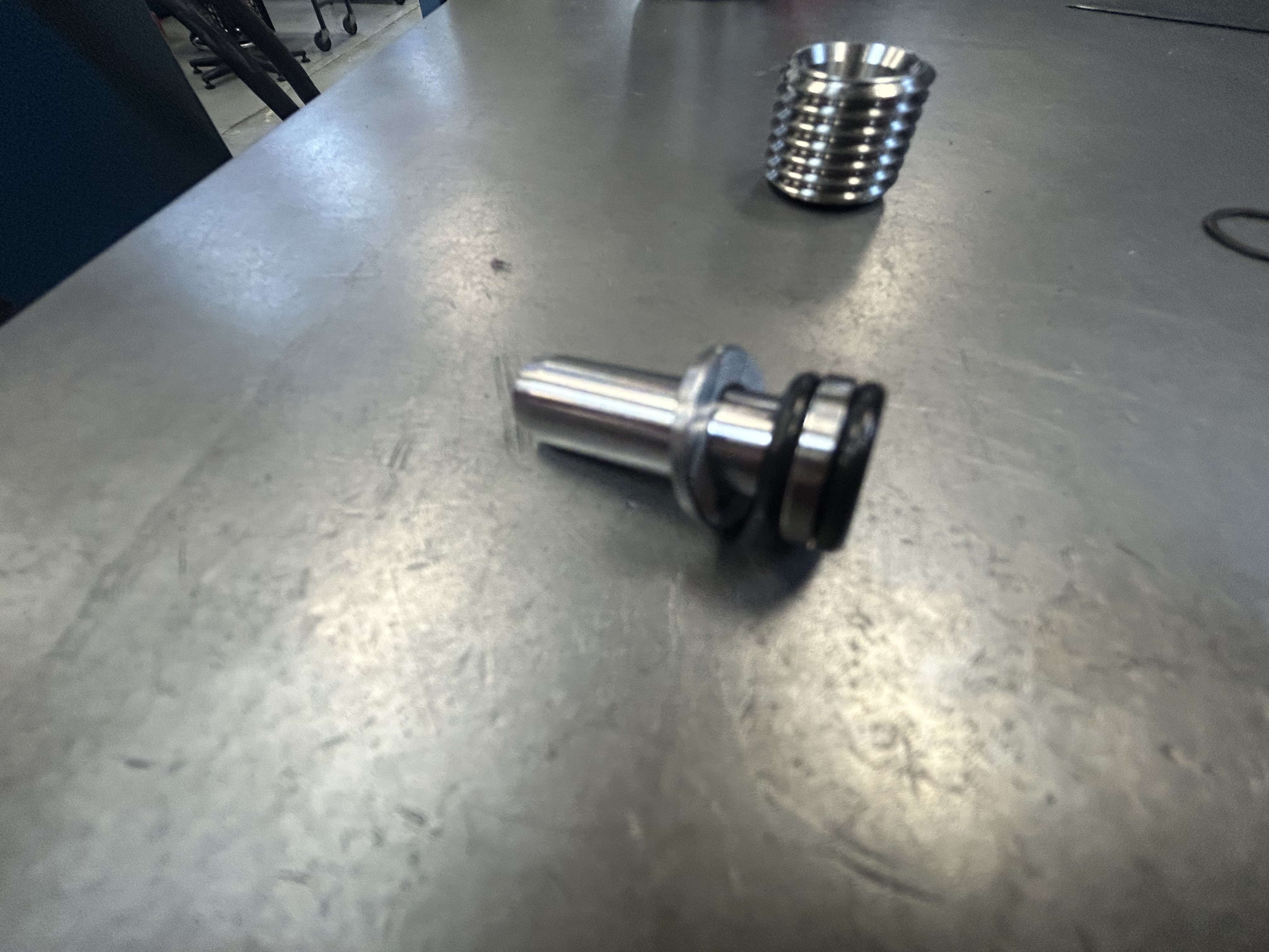
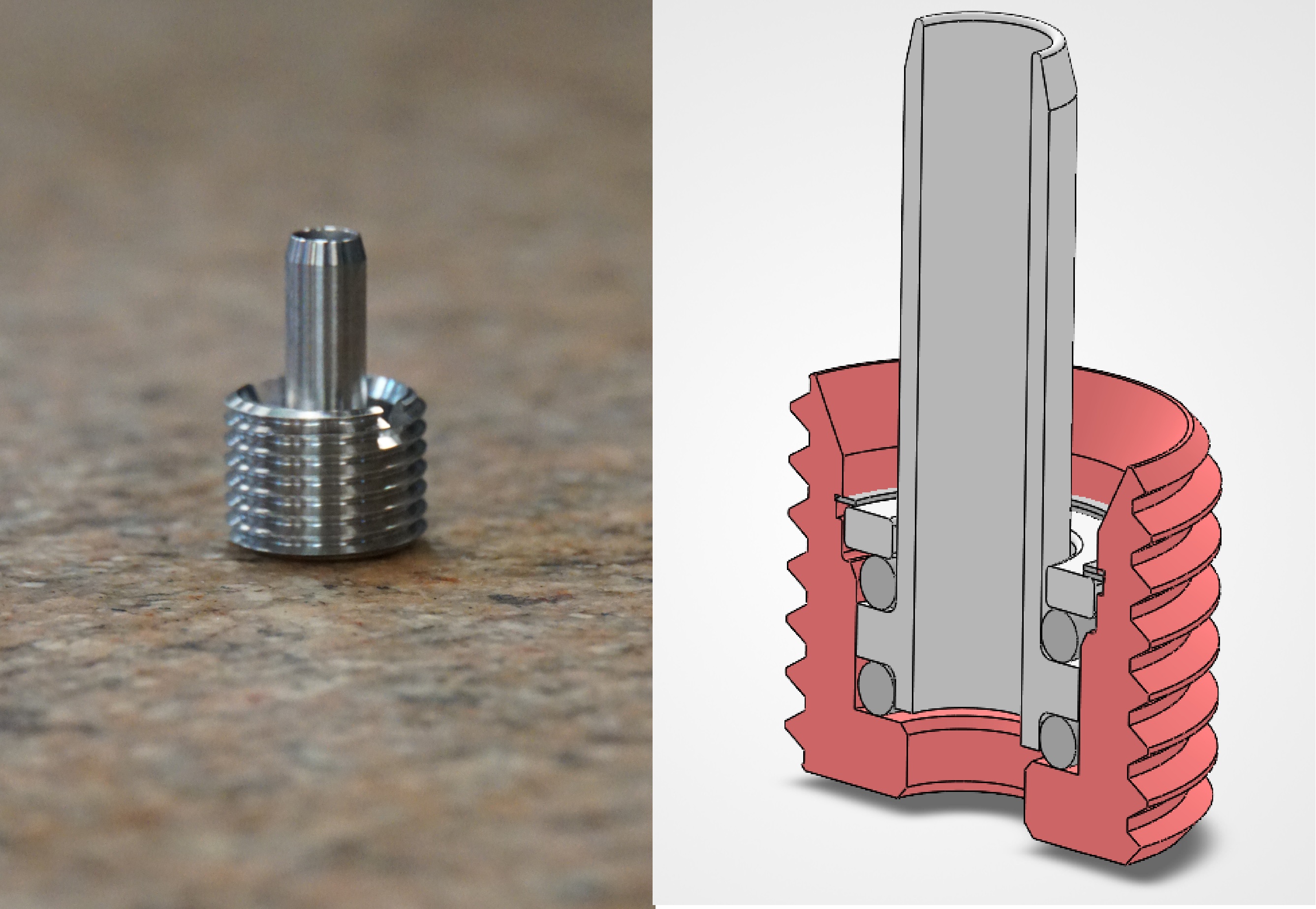
Machined Parts
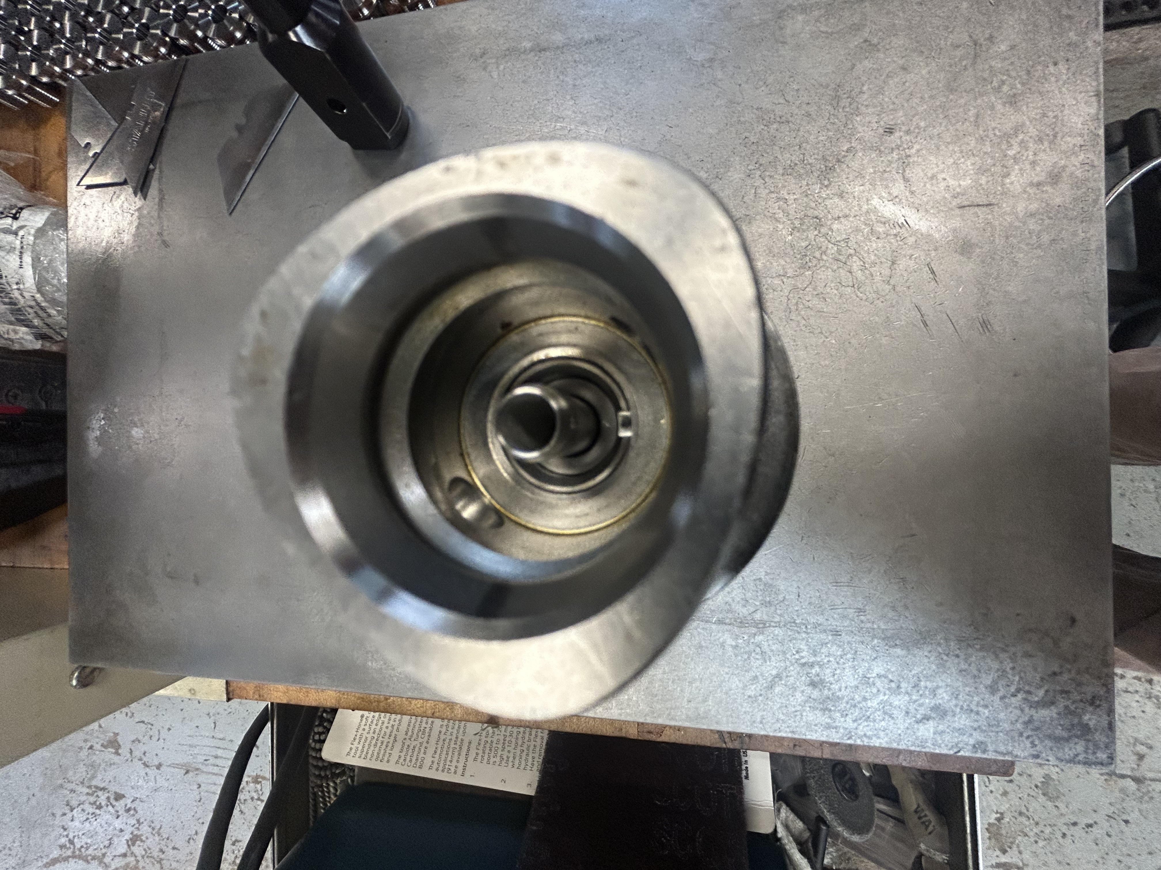
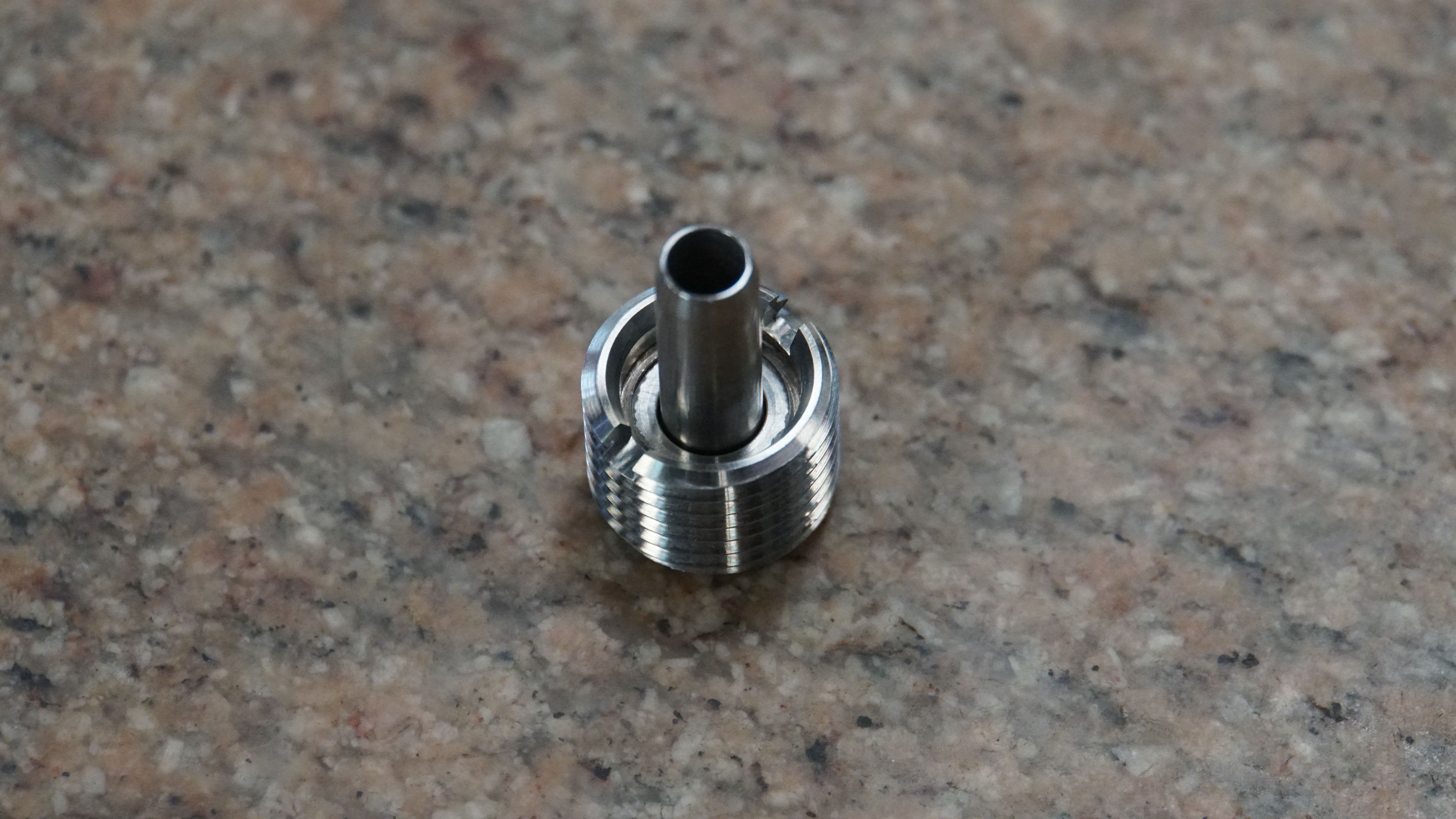
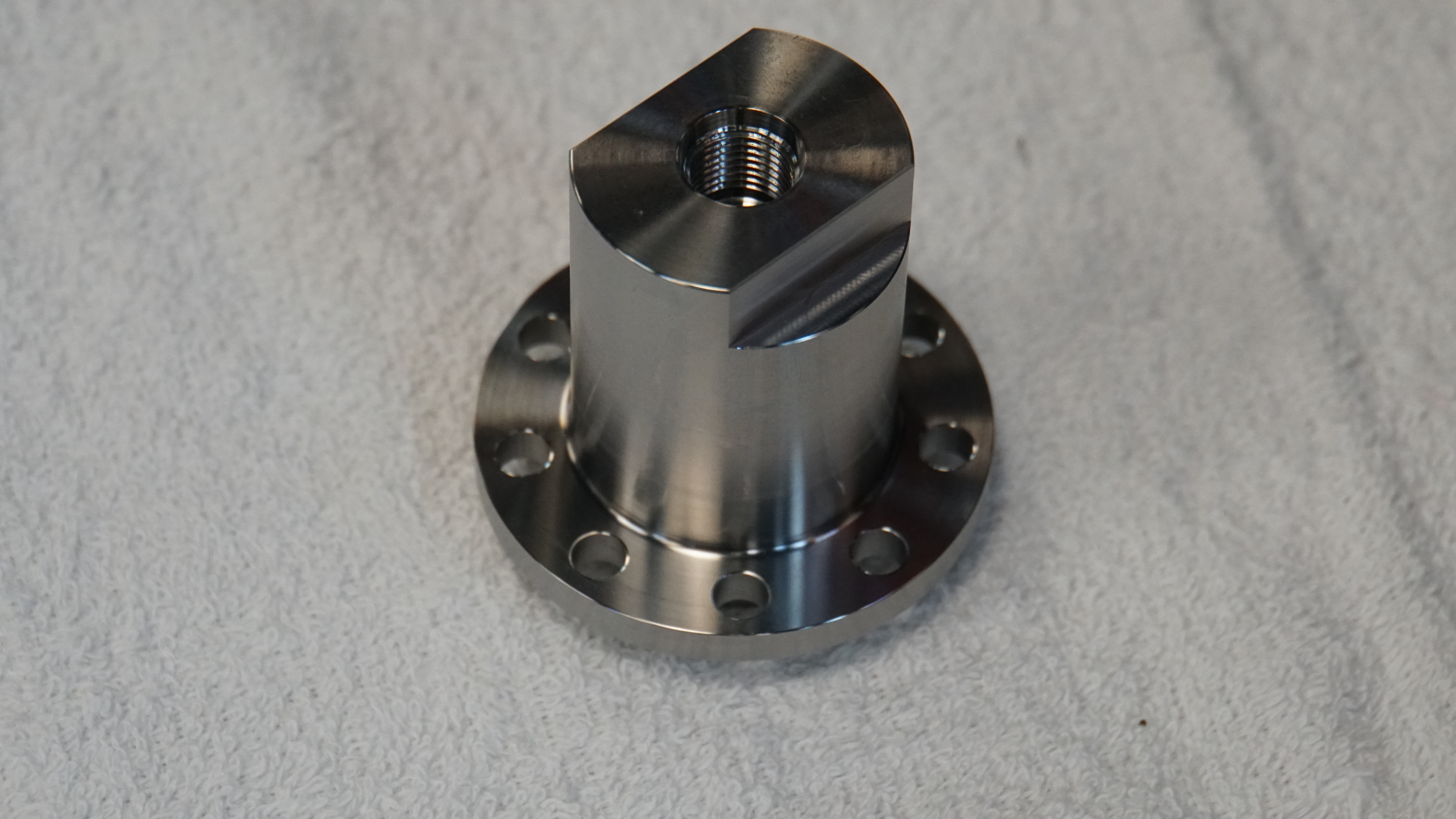
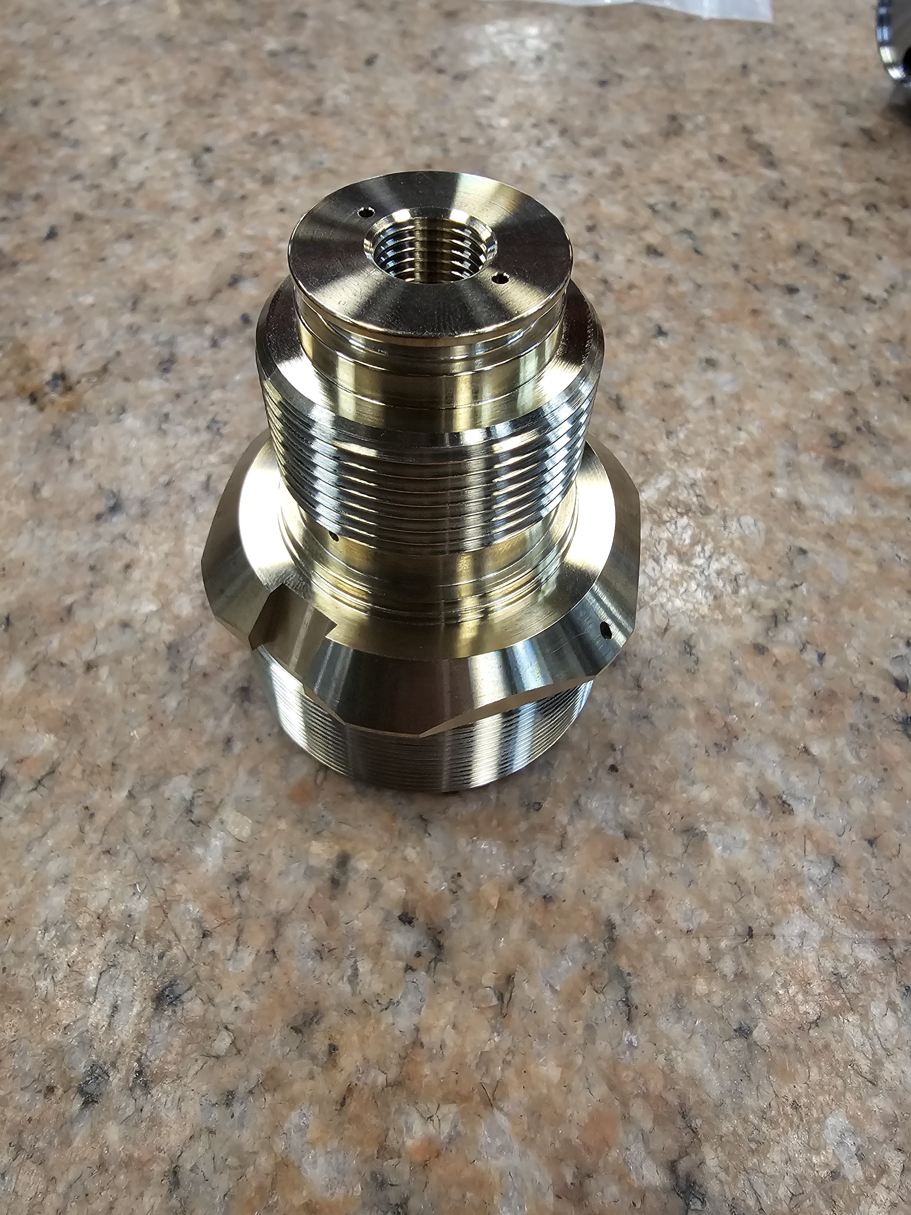
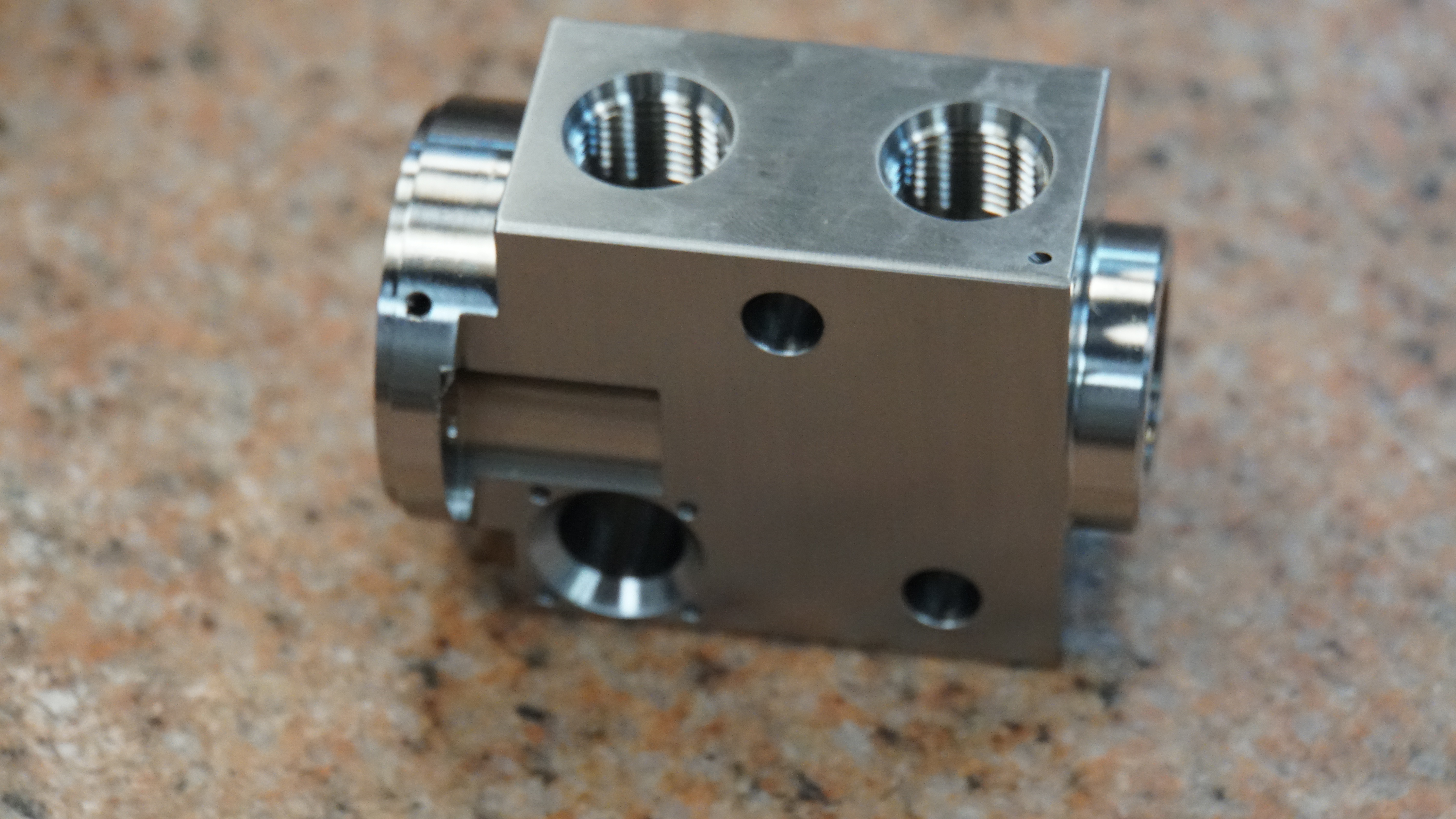
Machined precision components
Machined production components — photographed physical hardware from the project documentation.

Four-Part Manufacturing Portfolio

Part A: Multi-threaded brass fitting with turned/threaded features, live-tool geometry, and cross drilling.

Part B: Stainless flanged hub with bolt-circle features, internal threading, and milled geometry.

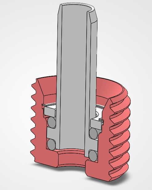
Part C (most complex): Stainless manifold-style component with multi-face features, ports/passages, and O-ring-related geometry.

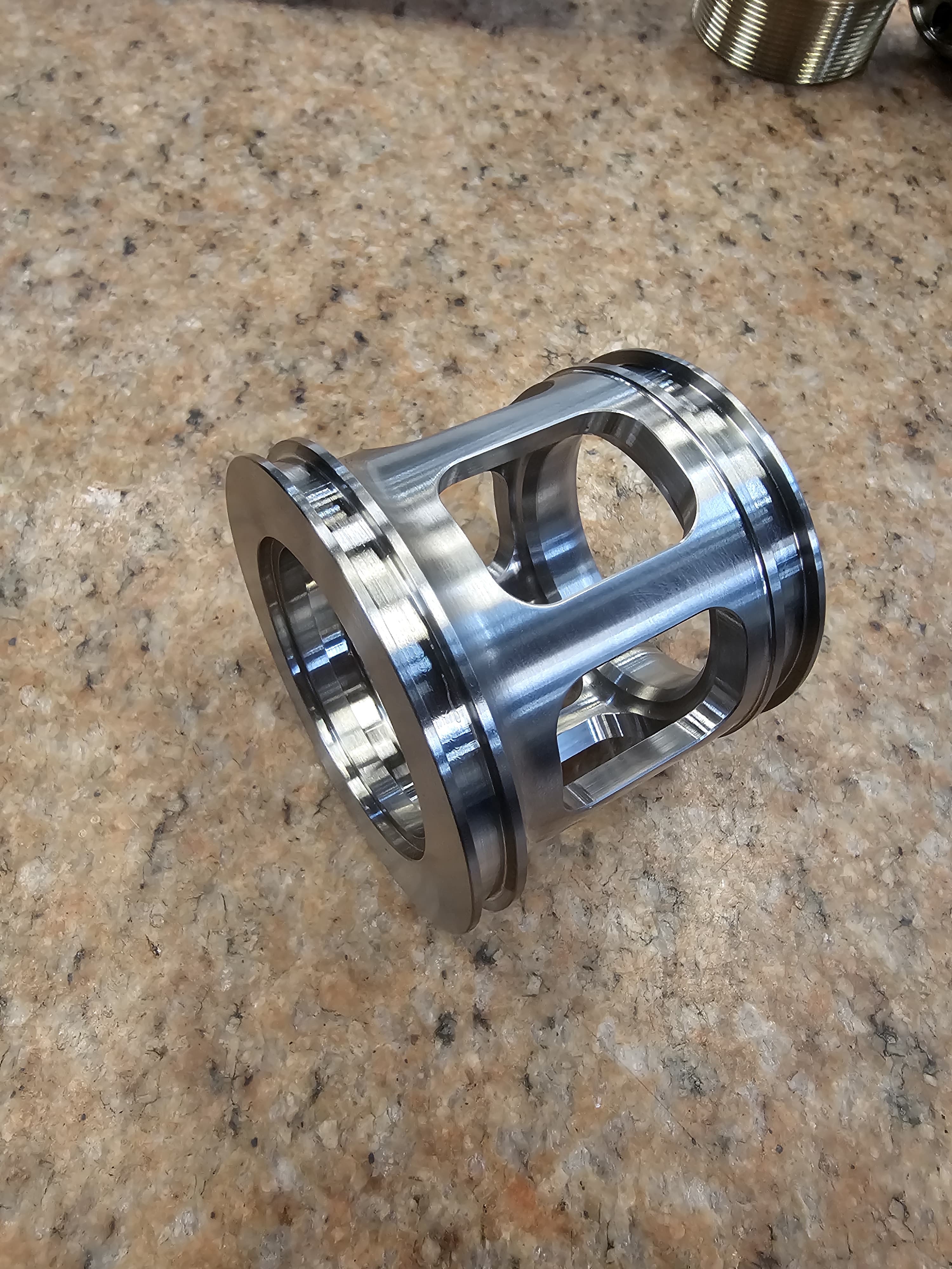
Part D: Thin-wall stainless cage/retainer with open windows requiring attention to deflection and concentricity.

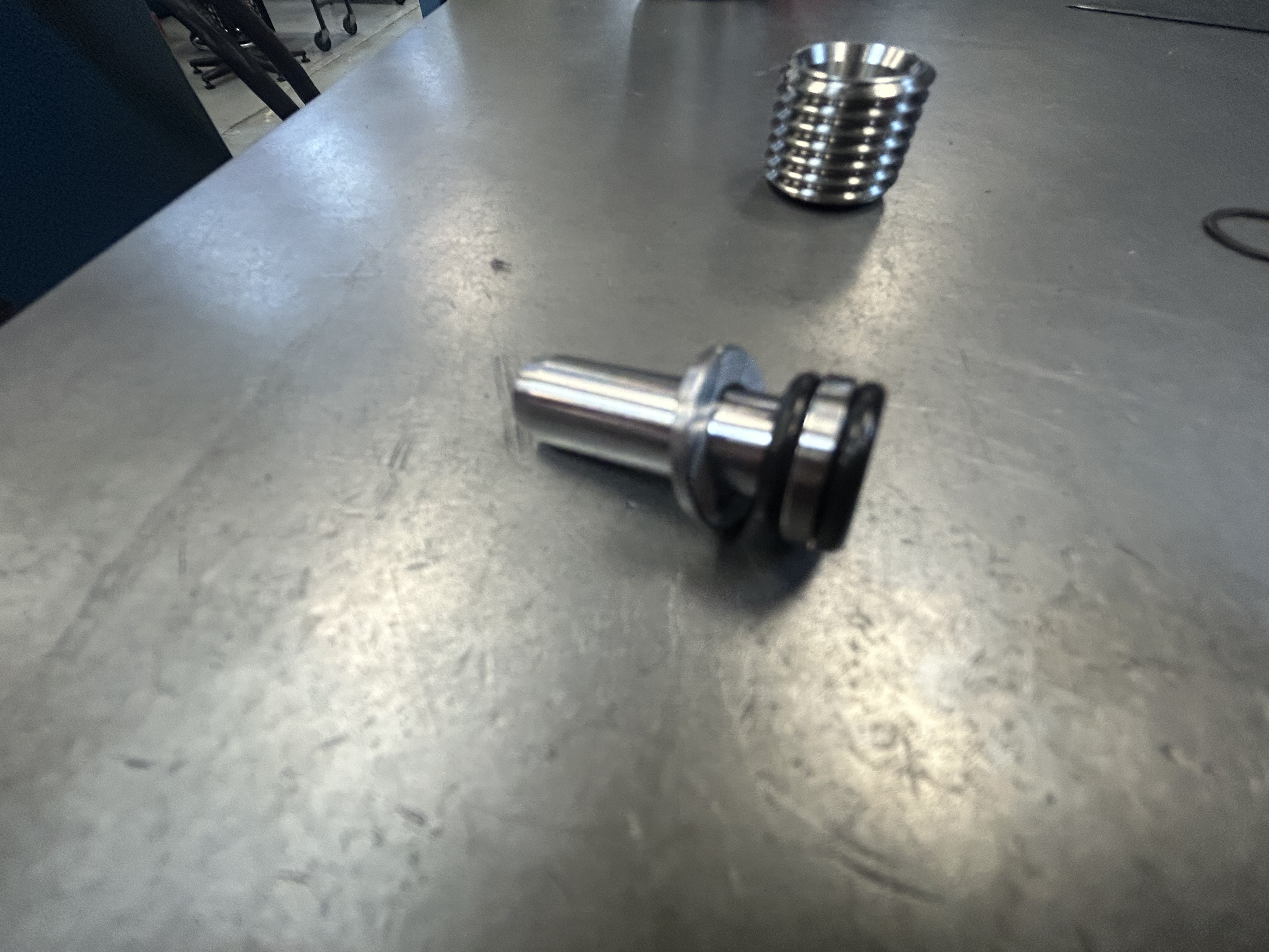
Additional machined parts
Additional machined components showing surface finish quality and geometric complexity.

Machines & Programming

  • Mazak INTEGREX i-200: multi-tasking / 5-axis-capable machine
  • Mazak turning/milling lathe: turning plus live-tool secondary operations
  • Hurco VMC: 3-axis vertical machining

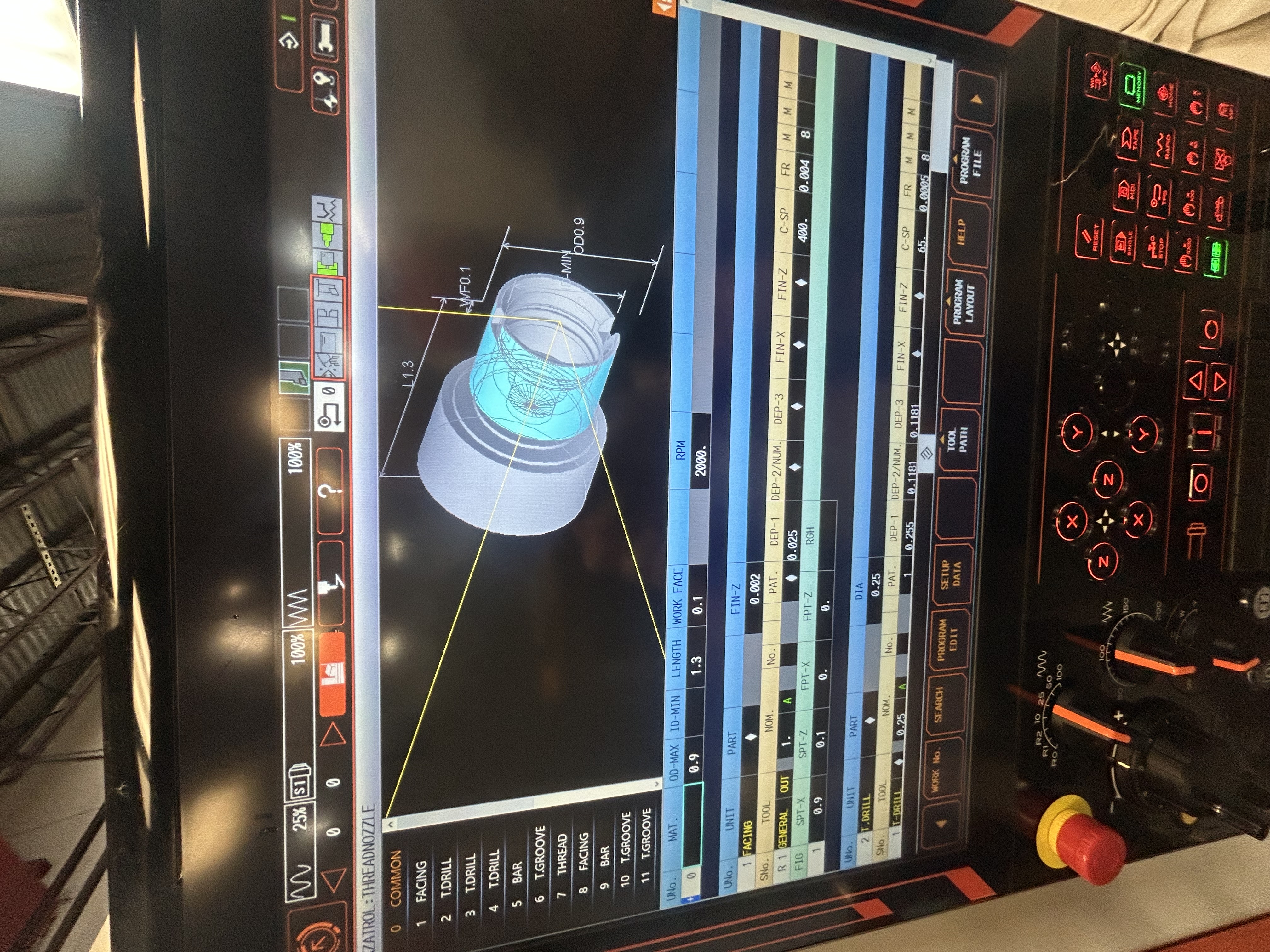
Programming exposure: MAZATROL conversational, G-code, and GibbsCAM multi-axis CAM.

Detailed view of machined component
Detail view — thread form quality and surface finish on a machined component.

Metrology & Inspection

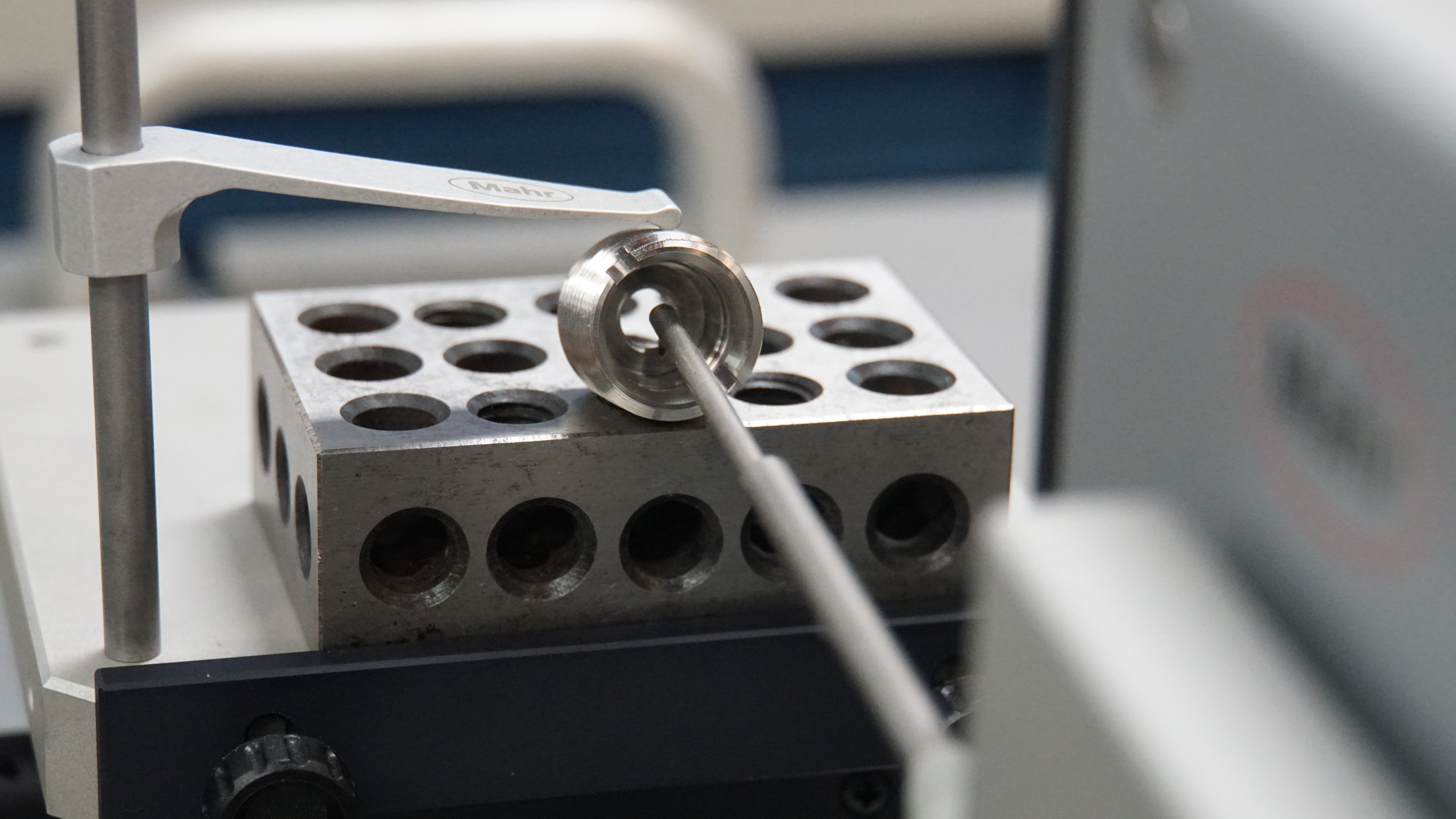
Project documentation records dimensional inspection using CMM and bench metrology including micrometers, calipers, thread gages, pin gages, optical comparison, and surface profilometry.

The project record contains 40 documented inspection characteristics reported within their stated limits with a 99% pass rate PROJECT RECORD.

Closeup of machined surface showing finish quality
Surface finish closeup — face-milled stainless steel; the best documented surface finish reached Ra 6.2 μin (0.16 μm).

Surface Finish

Surface-finish acceptance is drawing- and function-specific; the documented measurements demonstrate experience with profilometry and machining-process effects — Ra 6.2–36.4 μin across measured features.

For ideal turning geometry, Ra ≈ f²/(32r) and the approximate peak-to-valley theoretical height Rt ≈ f²/(8r) CALCULATED. For the documented brass example (f = 0.003 in/rev, r = 1/32 in): Ratheory ≈ 9 μin versus project-recorded Ra ≈ 16.2 μin — real finish also depends on material, tool condition, vibration, built-up edge, cutting speed, and machine dynamics.

Tolerance & Surface Analysis
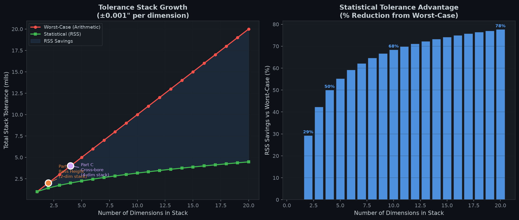
Tolerance-analysis method illustration
Tolerance-analysis method — worst-case (TWC = Σ|Ti|) and RSS (TRSS = √ΣTi²) approaches applied to assembly dimension chains.

Tolerance Stack Analysis

Worst-case and RSS (root-sum-square) tolerance-stack analysis was applied to assembly-critical dimension chains to understand how feature tolerances accumulate — a core manufacturing-design skill, since unnecessarily tight tolerances add cost without functional benefit.

Studied Cp/Cpk and SPC concepts as part of manufacturing-quality analysis; the available portfolio inspection set is not used to claim statistical process capability.

CNC Machining Multi-Axis Metrology / CMM GD&T / ASME Y14.5 Tolerance Analysis MAZATROL G-Code GibbsCAM
Project 06

Mortise Lock Reverse Engineering

Teardown → Measurement → SolidWorks Reconstruction → FDM Functional Prototype

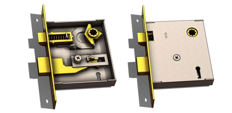
Complete reverse engineering of a commercial mortise lock — from systematic disassembly and precision measurement through parametric SolidWorks reconstruction and a functional FDM 3D-printed prototype.

10
Components
10
SLDPRT Files
6
Phase Workflow
Functional
Prototype
Assembly & Mechanism
SolidWorks reconstruction of the mortise-lock assembly
CONCEPT / RENDER SolidWorks reconstruction of the 10-component mortise-lock assembly.

Six-Phase Reverse-Engineering Workflow

  1. Disassembly with component cataloging
  2. Measurement with digital calipers
  3. CAD Modeling — 10 parametric SolidWorks component models
  4. STL / print preparation with FDM tolerance compensation
  5. FDM fabrication
  6. Functional validation of the reassembled mechanism

Assembly mates preserved the real kinematics (concentric, coincident, limit mates); design intent was inferred from measurement clusters rather than simply copying geometry.

Engineering Analysis
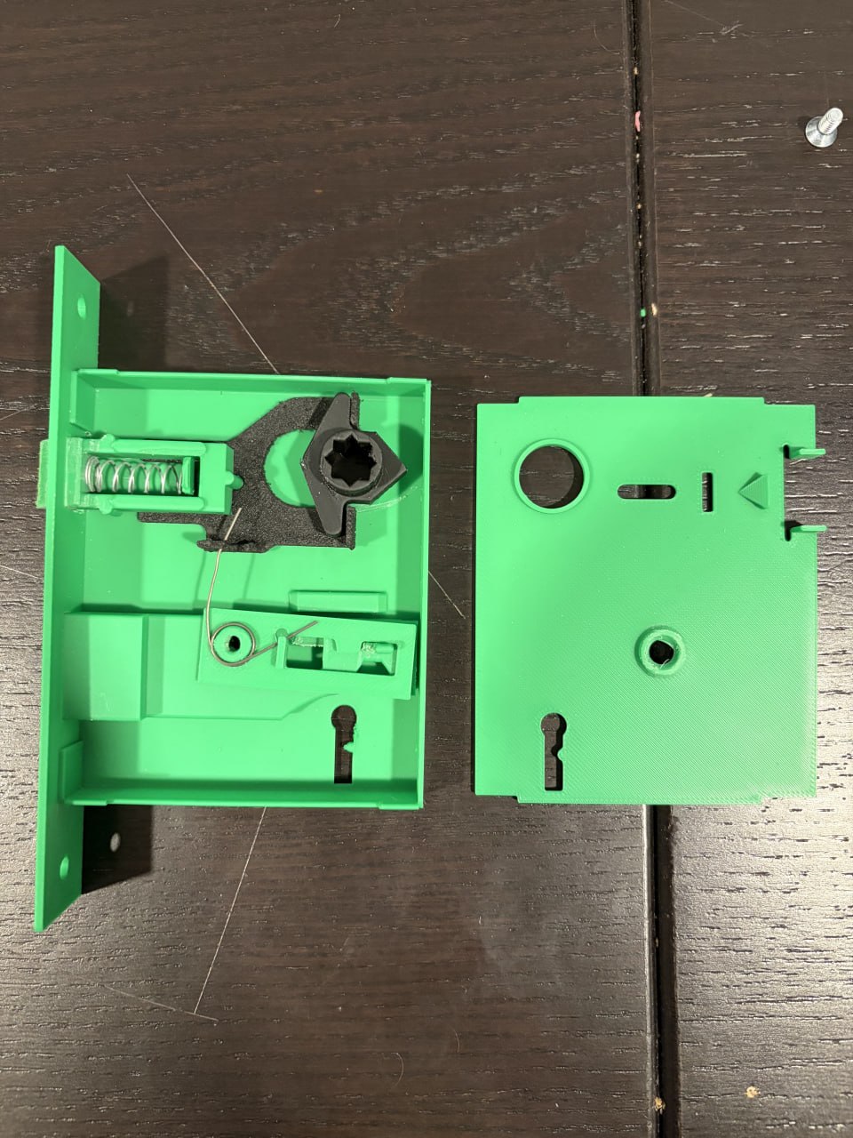
Actual mortise lock — physical hardware teardown reference
The actual mortise lock — physical hardware that was disassembled, measured, and reverse-engineered for this project.

Physical Hardware

The commercial mortise lock shown here was systematically disassembled, measured with digital calipers, and reconstructed as parametric SolidWorks models. Each component was cataloged and individually modeled to preserve the full assembly kinematics.

Latch return spring analysis
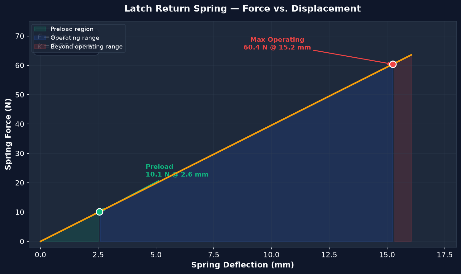
Latch return spring analysis — helical compression-spring rate derived from measured geometry.

Spring Analysis

Spring rate from the helical compression formula k = Gd⁴/(8D³Na) with d = 0.80 mm, D = 5.55 mm, Na = 6, and G = 79.3 GPa CALCULATED ASSUMPTION (material):

  • k ≈ 3.96 N/mm
  • Preload ≈ 10.10 N
  • Max modeled spring load ≈ 60.39 N

Shear modulus and material properties come from handbook values, not a material certificate for this specific spring.

Cam Kinematics — Deadbolt Actuation

A simplified eccentric-cam model reproduces the measured approximately 15.88-mm deadbolt throw over approximately 90° of key rotation CALCULATED:

s(θ) = e ( 1 − cos θ ),   e = 15.88 mm
s(90°) = 15.88 mm

The model captures the displacement relationship as documented; no force-amplification claim is made without a defined input torque and lever geometry.

Material substitution comparison — steel vs PLA
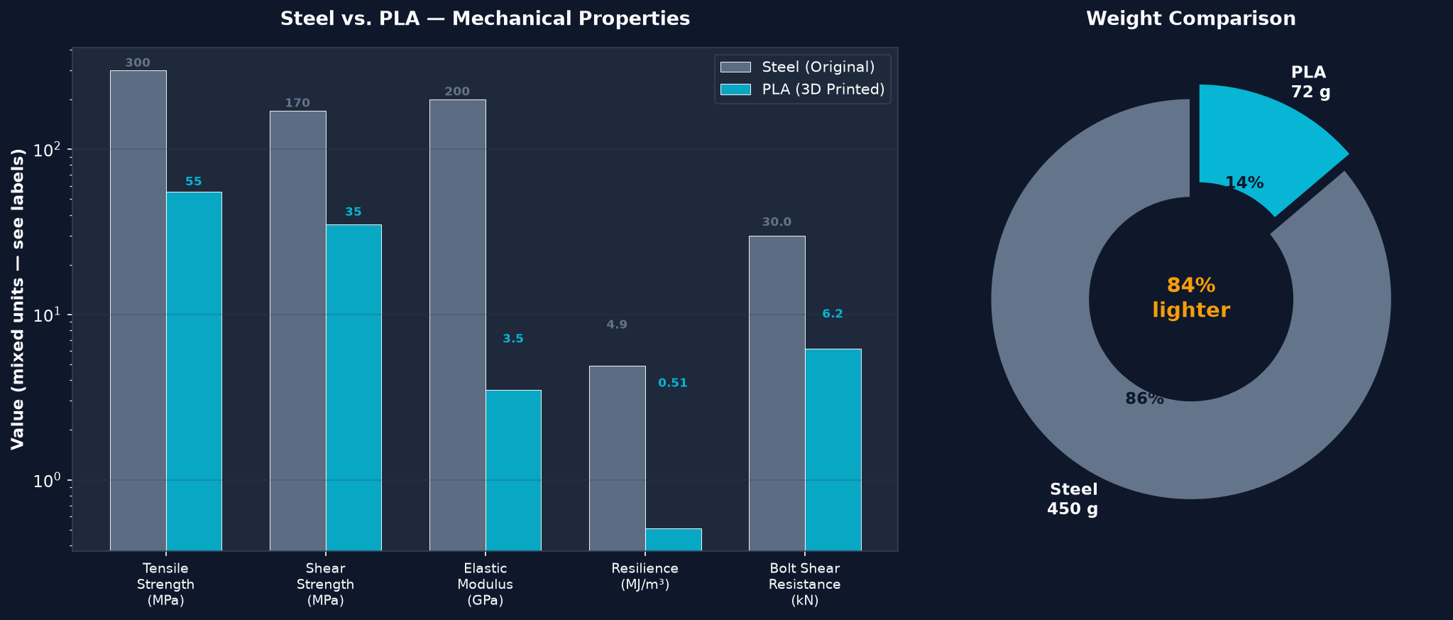
ANALYTICAL ASSUMED Illustrative material-substitution comparison using representative material-property assumptions and estimated component weights.

Material Substitution

Under representative material-strength assumptions, the printed PLA deadbolt has approximately 21% of the modeled steel deadbolt shear capacity (6.2 kN vs 30.0 kN). This is an analytical material-substitution estimate, not a security rating or a destructive test ASSUMPTION.

Estimated assembly masses: steel ≈450 g, printed PLA ≈72 g — both estimates, not measured weights.

The PLA latch bevel was increased from 15° to 25° for self-retraction margin: the screening criterion tan(α) > μ was applied with representative PLA-on-steel friction used as a screening assumption, not measured on the printed surface. The final prototype was documented as functioning after post-processing.

Handle Force — Simplified Lever Statics

With lever-arm ratio r2/r1 = 22.0/8.5 ≈ 2.59 and the maximum modeled spring force of 60.39 N CALCULATED:

Fhandle = Fspring × ( r1 / r2 ) ≈ 23.3 N

Simplified lever statics predicts approximately 23.3 N maximum handle force under the modeled spring load (and ≈1.28 N·m torque at the documented handle radius). This is a statics exercise, not ergonomic validation.

CAD-to-print dimensional comparison
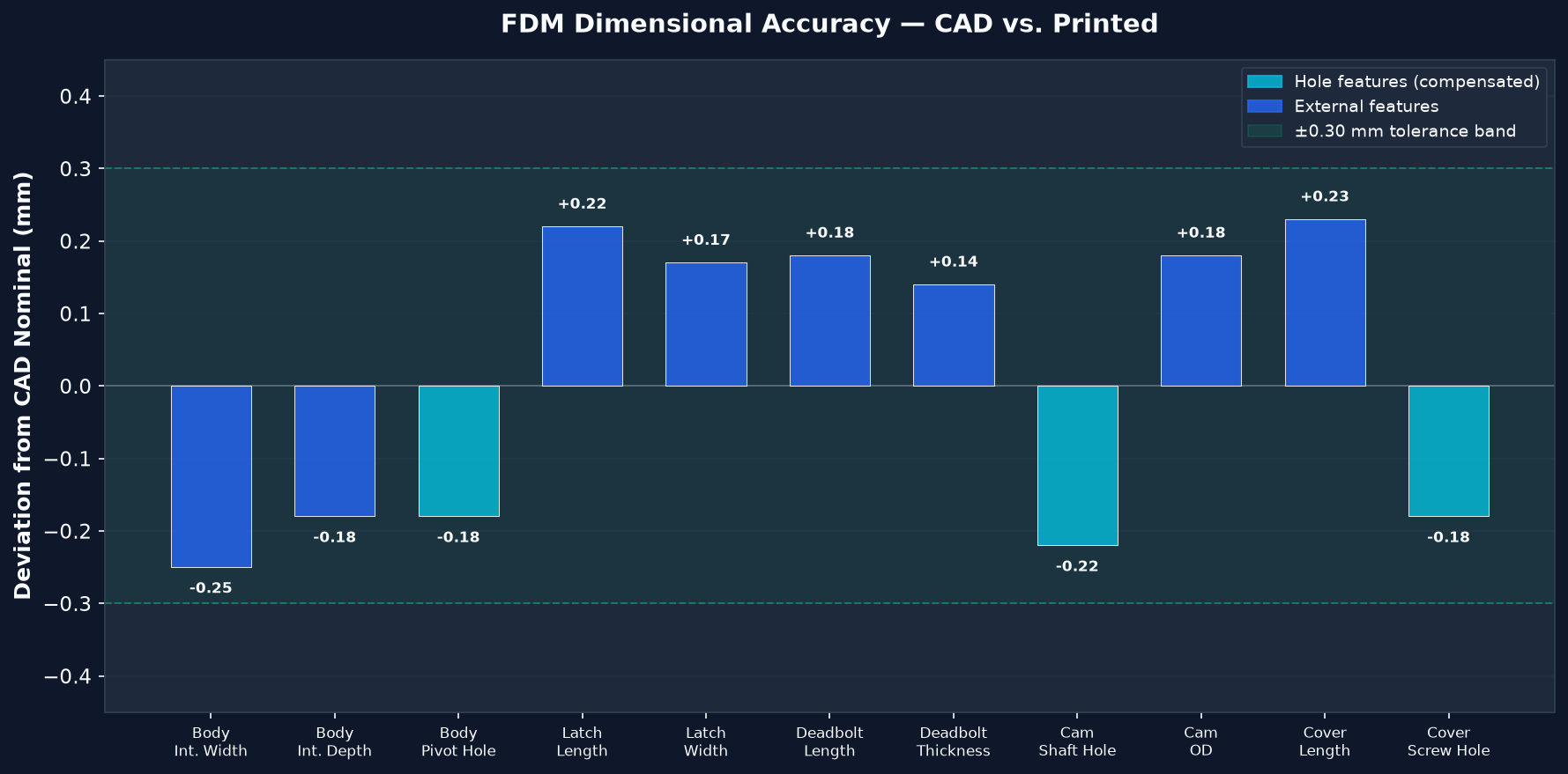
Project-recorded CAD-to-print dimensional comparison.

FDM Dimensional Accuracy

Observed dimensions in the documented sample fell within the project's ±0.30-mm prototype fit target, with documented deviations on the order of approximately ±0.25 mm PROJECT RECORD. This describes the documented sample only, not universal FDM process capability.

Holes and shaft fits were compensated (+0.2–0.4 mm) during print preparation to accommodate FDM shrinkage and layer artifacts.

This project demonstrates teardown-driven reverse engineering, parametric CAD reconstruction, mechanism analysis, material/process substitution, FDM tolerance compensation, and functional reassembly.

Reverse Engineering SolidWorks CAD Mechanism Design FDM 3D Printing Cam Kinematics Material Substitution

Engineering Competencies

A cross-section of capabilities demonstrated across six projects — from CNC machining and CAD modeling to embedded systems and machine learning.

⚙

Manufacturing & CNC

  • CNC Turning & Milling (3–5 axis)
  • MAZATROL Conversational Programming
  • G-Code (ISO 6983)
  • GibbsCAM Multi-Axis
  • Single-Point Threading
  • Thin-Wall & Multi-Face Machining
  • Blueprint Reading (ASME Y14.5)
📊

Metrology & Quality

  • CMM Inspection / Operation
  • GD&T (ASME Y14.5-2018)
  • Tolerance Analysis / Statistical Quality Concepts
  • Surface Profilometry (Mahr MarSurf)
  • Micrometer / Caliper / Pin Gage
  • Thread Gaging (Go/No-Go)
  • Measurement Uncertainty Analysis
⚿

CAD & Design

  • SolidWorks Parametric Modeling
  • Part & Assembly Design
  • Reverse Engineering
  • Design for Manufacturability (DFM)
  • Tolerance Stack Analysis
  • GD&T Callouts
  • Engineering Drawings
💻

Controls & Embedded

  • PID Control (Tuning & Implementation)
  • Sensor Fusion (Complementary Filter)
  • Arduino / ATmega328P
  • MATLAB / Simulink
  • Real-Time Embedded Systems
  • Stepper Motor Control (A4988)
  • I2C / SPI / UART Communication
🧮

Analysis & Simulation

  • SolidWorks Simulation / Python Stress Analysis
  • Fluid Dynamics (Bernoulli, Darcy-Weisbach)
  • Structural Analysis (Lamé, Von Mises)
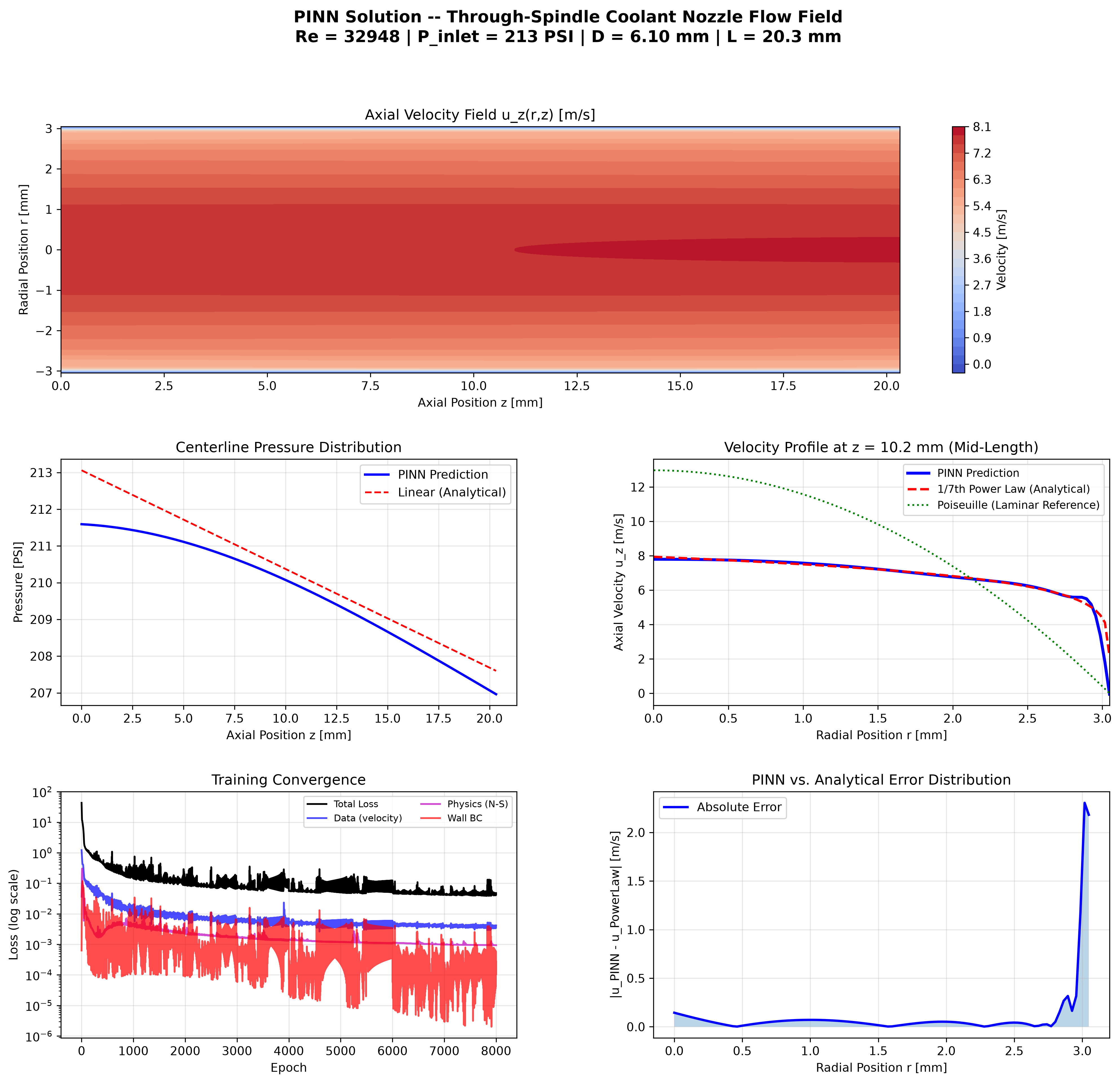
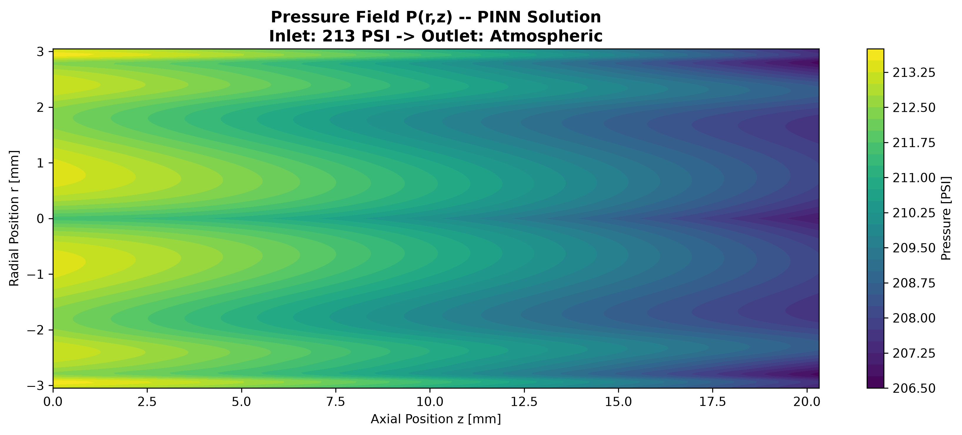
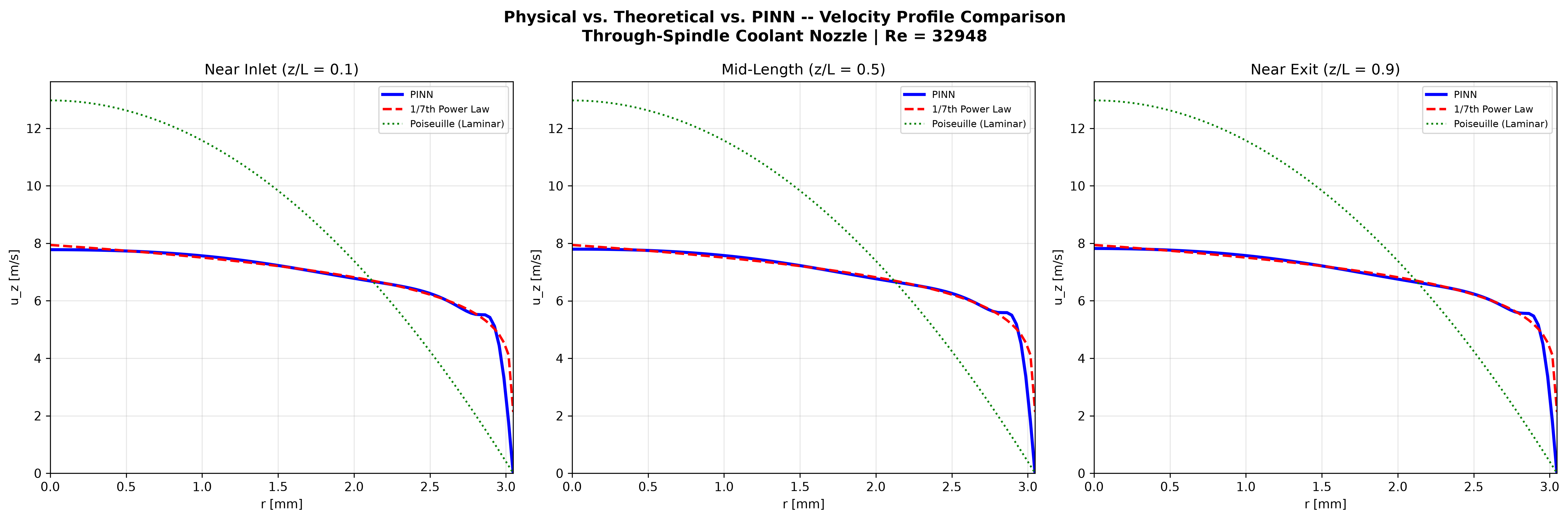
  • Physics-Informed Neural Networks (PINN)
  • Signal Processing (PPG, FFT, Filtering)
  • Statistical Error Analysis
  • FMEA (Failure Mode & Effects)
🔬

Tools & Software

  • Python (PyTorch, NumPy, Matplotlib)
  • SolidWorks + SolidWorks Flow Sim
  • GibbsCAM
  • Git / Version Control
  • Microsoft Excel (Data Analysis)
  • Arduino IDE